
通知设置 新通知
抄底?还是跳入火坑
股票 • 绫波丽 发表了文章 • 0 个评论 • 3561 次浏览 • 2018-04-27 20:54
截几个图给大家看看:
富控互动(点击查看大图)
如果你去抄底了,在图示2的位置买入,假如你买入1W快,那么到今天(2018-04-27)如果没及时止损割肉,那么现在就剩6900.
而如果是从1的位置买入一直持有到现在,那么现在就剩4000元。
顺威股份(点击大图)
如果你在2位置抄底,那么现在会亏损40%
同样,如果你在2位置去抄底神雾
那么到现在你会亏损51%,而在3位置去抄底,那么你到现在会亏损31%,所以抄底过程中,如果你没有做好马上捞一笔就跑的习惯,还是不要去参与。参与了,就要跑的快,不论盈利或者亏损。 不然后面的都是深渊。
查看全部
截几个图给大家看看:

富控互动(点击查看大图)
如果你去抄底了,在图示2的位置买入,假如你买入1W快,那么到今天(2018-04-27)如果没及时止损割肉,那么现在就剩6900.
而如果是从1的位置买入一直持有到现在,那么现在就剩4000元。

顺威股份(点击大图)
如果你在2位置抄底,那么现在会亏损40%
同样,如果你在2位置去抄底神雾

那么到现在你会亏损51%,而在3位置去抄底,那么你到现在会亏损31%,所以抄底过程中,如果你没有做好马上捞一笔就跑的习惯,还是不要去参与。参与了,就要跑的快,不论盈利或者亏损。 不然后面的都是深渊。
统计下各种券商的股票,债券,场内ETF基金,逆回购等手续费率
券商万一免五 • 绫波丽 发表了文章 • 0 个评论 • 7286 次浏览 • 2018-04-26 23:24
现在总结一些,可以给大家参考:
华泰证券:
股票:万分之1.5
可转债(沪深市):万分之5
EFT基金:万分之3
国金证券:
股票:万分之1
可转债(新规)沪,深:十万分之4.4
海通证券:
股票:万分之1.5
可转债(深市):万分之5
==========
万一免5开户链接
==========
另外一个券商:
如果电脑浏览器打不开(只兼容手机端)可以扫描下面二维码开户: 查看全部
现在总结一些,可以给大家参考:
华泰证券:
股票:万分之1.5
可转债(沪深市):万分之5
EFT基金:万分之3
国金证券:
股票:万分之1
可转债(新规)沪,深:十万分之4.4
海通证券:
股票:万分之1.5
可转债(深市):万分之5
==========
万一免5开户链接
==========
另外一个券商:

如果电脑浏览器打不开(只兼容手机端)可以扫描下面二维码开户:

pandas中diff控制移动方向,向上移动
python • 李魔佛 发表了文章 • 0 个评论 • 6346 次浏览 • 2018-04-25 20:39
然后使用默认的diff(periods=1)
行的索引不变,数据被往下拉了一行。当然你也可以使用periods=2 ,那么数据整体会往下移2格。
如果要往上移动,只要把periods的值设为负的就可以了。
查看全部

初始化一个dataframe
然后使用默认的diff(periods=1)

行的索引不变,数据被往下拉了一行。当然你也可以使用periods=2 ,那么数据整体会往下移2格。
如果要往上移动,只要把periods的值设为负的就可以了。

树莓派中使用matplotlib出错 TypeError: constructor returned NULL
树莓派 • 李魔佛 发表了文章 • 0 个评论 • 6217 次浏览 • 2018-04-23 23:21
_backend_mod, new_figure_manager, draw_if_interactive, _show = pylab_setup()
File "/usr/local/lib/python2.7/dist-packages/matplotlib/backends/__init__.py", line 32, in pylab_setup
globals(),locals(),[backend_name],0)
File "/usr/local/lib/python2.7/dist-packages/matplotlib/backends/backend_gtk3agg.py", line 11, in <module>
from . import backend_gtk3
File "/usr/local/lib/python2.7/dist-packages/matplotlib/backends/backend_gtk3.py", line 54, in <module>
cursors.MOVE : Gdk.Cursor.new(Gdk.CursorType.FLEUR),
TypeError: constructor returned NULL
上面的代码是在树莓派上运行出错的,而在本地的ubuntu上正常运行没问题。
后面查了下资料,原因是我用了ssh登录到树莓派,所以X11的模块没有被正常加载。
按照以下方法就可以解决问题了:
在代码中添加以下这一句:
matplotlib.use("Pdf")
而且这一句要在import matplotlib.pyplot as plt这句前面添加。
OK。 查看全部
 File "/usr/local/lib/python2.7/dist-packages/matplotlib/pyplot.py", line 115, in <module>

    _backend_mod, new_figure_manager, draw_if_interactive, _show = pylab_setup()

  File "/usr/local/lib/python2.7/dist-packages/matplotlib/backends/__init__.py", line 32, in pylab_setup

    globals(),locals(),[backend_name],0)

  File "/usr/local/lib/python2.7/dist-packages/matplotlib/backends/backend_gtk3agg.py", line 11, in <module>

    from . import backend_gtk3

  File "/usr/local/lib/python2.7/dist-packages/matplotlib/backends/backend_gtk3.py", line 54, in <module>

    cursors.MOVE          : Gdk.Cursor.new(Gdk.CursorType.FLEUR),

TypeError: constructor returned NULL
上面的代码是在树莓派上运行出错的,而在本地的ubuntu上正常运行没问题。
后面查了下资料,原因是我用了ssh登录到树莓派,所以X11的模块没有被正常加载。
按照以下方法就可以解决问题了:
在代码中添加以下这一句:
matplotlib.use("Pdf")
而且这一句要在import matplotlib.pyplot as plt这句前面添加。
OK。
python安装mpl_finance [finance模块已经从matplotlib2.0.2中脱离出来]
python • 李魔佛 发表了文章 • 0 个评论 • 19675 次浏览 • 2018-04-23 23:17
解决办法:
到官方github中下载源码,然后在本地安装即可。 目前的mpl_finance的版本还是dev版,不过用起来也没什么大问题。
git clone git@github.com:matplotlib/mpl_finance.git
等待下载后,进入该目录, sudo python setup.py install
OK
查看全部
解决办法:
到官方github中下载源码,然后在本地安装即可。 目前的mpl_finance的版本还是dev版,不过用起来也没什么大问题。
git clone git@github.com:matplotlib/mpl_finance.git
等待下载后,进入该目录, sudo python setup.py install
OK
jupyter notebook 数据分析的利器
每日总结 • 李魔佛 发表了文章 • 0 个评论 • 3656 次浏览 • 2018-04-22 15:33
而且很重要的一点,jupyter使用web 服务器的方式运行,可以在树莓派上开一个jupyter服务,然后配置一下,就可以在其他的电脑上通过浏览器运行jupyter。 其他电脑不必要安装任何python和配置虚拟环境。 查看全部
而且很重要的一点,jupyter使用web 服务器的方式运行,可以在树莓派上开一个jupyter服务,然后配置一下,就可以在其他的电脑上通过浏览器运行jupyter。 其他电脑不必要安装任何python和配置虚拟环境。
Coinegg需要VPN才能访问
量化交易 • 李魔佛 发表了文章 • 0 个评论 • 2954 次浏览 • 2018-04-22 00:17
好久没上去看,成交了太稀疏了。

好久没上去看,成交了太稀疏了。
俗语“十赌九输” 是真的吗 ? 赌场第一定律,庄家永远不会告诉你
股票 • 李魔佛 发表了文章 • 0 个评论 • 17088 次浏览 • 2018-04-17 00:20
在赌场上,常常听到一句劝人原理赌场的话:“十赌九输”,那么这句话是真的吗?
如果有庄家佣金抽成,那么很多人都知道,最后的赢家就是庄家,因为每玩一局,就会产生摩擦资金,比如2个人玩在骰子的大小,输赢50%的概率,假如每局都要交1%押注资金给庄家,那么两个人即使是你的钱进我口袋,我的钱进你口袋,但是两个人的资金总和是在不断减少。 这种是赌场最常见的情形,大部分人有数学能力的人也都能认清,所以大部分清醒的人不太会参与这样的赌场。
假如赌场没有佣金抽成,而且输赢的概率都是50%呢? 这样是不是最后会一直可以玩下去呢? 答案是否定的。
数学理解:
赢多了一定有输回来的概率。
但输光了,却没有再赢回来的资本。
咱们仅讨论概率,假设赌博绝对公平,每场五成概率+1,五成概率-1。
下面用代码模拟这个赌博的过程。
假设初始赌资为100,每次下注为1,赢了100+1, 输了100-1, 一直循环下去,直到赌资等于0,输精光出局,赢得话就一直玩下去,每次下注金额固定为1。
为了更加清晰的对比初始赌资和赌博次数的关系,我们把赌资从1开始到100,最后的赌博次数情况。
如果你的赌资是1,每局下注1,那么这种情况很可能你玩1局就挂掉了,如果赌资是100,根据平均大数定律,就可以无限地玩下去,因为连续出100个小的概率非常低,是这样吗?
为了得到更为普遍的结果,每一个赌资运行5次,得到的结果取平均值,这样可以有效取出奇异值,如果想要结果更为精确,可以每一个赌资运行10次甚至100次,不过这个过程也稍微更加耗时。
最后得到的数据如下,最终程序是可以收敛,结束了,就是赌资从1到100,每次下注1 , 50%的输赢概率,最终都输精光离场,不同的只是你呆在场上的时间。 最长的可以玩3千多万局,最低的玩6局离场,也就是1元赌资标号的那位。 [6.2, 20.4, 18.6, 20.0, 1366.2, 117.2, 609.4, 237.2, 407.0, 798.8, 1324.6, 46327.6, 81275.4, 1604854.8, 11903.0, 24018.8, 783.8, 27538.8, 867.4, 2291.2, 3753.0, 10562.0, 6540.6, 3519988.4, 15201.8, 405.2, 135648.2, 101014.8, 15703.4, 5506.0, 5369.0, 7870.0, 3815.0, 8325712.4, 23636.6, 1556.8, 95365.8, 1262.4, 625404.2, 6300430.8, 126025.0, 31276.0, 28717.4, 23184.0, 29007.4, 20586.0, 4581.0, 10091574.4, 111960.6, 3848.0, 1643635.4, 135605.6, 80114.2, 12795.2, 14133.4, 724014.4, 5365.4, 12682.8, 7472.2, 10351.6, 35163.8, 542070.8, 22053.0, 6292.4, 83359.4, 15030.8, 45987.8, 114825.2, 3121.4, 609555.6, 1307542.6, 8402.4, 62410.2, 231369.6, 285103.8, 660060.4, 719555.8, 69072.0, 41764.6, 181634.8, 40792.2, 57721.2, 59925.8, 134405.6, 41730.6, 62014.0, 1200179.8, 32587184.0, 5717.4, 13583.2, 24479.4, 339389.2, 12449571.4, 29882201.2, 2729118.6, 942646.8, 37097.8, 4795026.0, 359242.2]
为了更为直观,绘制成图形。
点击查看原图
横坐标为赌资的大小,纵坐标为赌博的次数。
因为纵坐标的某些次数极大,所以在图形中变成了凸起来的尖峰,不过普遍都是在5百万次以下。
这也间接说明,资金仓位管理的重要性,赌博总归是要归零的,如果你赌资足够大,或者每次下注小一些,每次小赌一下,那么你还是可以玩很久的,当然这是在公平50%的输赢概率上,但是如果输赢概率低于50%,那么,其收敛速度会急速下降,也就是加速你的离场速度。其他条件不变,上面的例子下进行赌博,那么100的赌资,平均下来大概也就能玩500局。
珍爱生命,远离赌博!!
原文链接:http://30daydo.com/article/292
转载请注明出处
查看全部
在赌场上,常常听到一句劝人原理赌场的话:“十赌九输”,那么这句话是真的吗?
如果有庄家佣金抽成,那么很多人都知道,最后的赢家就是庄家,因为每玩一局,就会产生摩擦资金,比如2个人玩在骰子的大小,输赢50%的概率,假如每局都要交1%押注资金给庄家,那么两个人即使是你的钱进我口袋,我的钱进你口袋,但是两个人的资金总和是在不断减少。 这种是赌场最常见的情形,大部分人有数学能力的人也都能认清,所以大部分清醒的人不太会参与这样的赌场。
假如赌场没有佣金抽成,而且输赢的概率都是50%呢? 这样是不是最后会一直可以玩下去呢? 答案是否定的。
数学理解:
赢多了一定有输回来的概率。
但输光了,却没有再赢回来的资本。
咱们仅讨论概率,假设赌博绝对公平,每场五成概率+1,五成概率-1。
下面用代码模拟这个赌博的过程。
假设初始赌资为100,每次下注为1,赢了100+1, 输了100-1, 一直循环下去,直到赌资等于0,输精光出局,赢得话就一直玩下去,每次下注金额固定为1。
为了更加清晰的对比初始赌资和赌博次数的关系,我们把赌资从1开始到100,最后的赌博次数情况。
如果你的赌资是1,每局下注1,那么这种情况很可能你玩1局就挂掉了,如果赌资是100,根据平均大数定律,就可以无限地玩下去,因为连续出100个小的概率非常低,是这样吗?

为了得到更为普遍的结果,每一个赌资运行5次,得到的结果取平均值,这样可以有效取出奇异值,如果想要结果更为精确,可以每一个赌资运行10次甚至100次,不过这个过程也稍微更加耗时。
最后得到的数据如下,最终程序是可以收敛,结束了,就是赌资从1到100,每次下注1 , 50%的输赢概率,最终都输精光离场,不同的只是你呆在场上的时间。 最长的可以玩3千多万局,最低的玩6局离场,也就是1元赌资标号的那位。
[6.2, 20.4, 18.6, 20.0, 1366.2, 117.2, 609.4, 237.2, 407.0, 798.8, 1324.6, 46327.6, 81275.4, 1604854.8, 11903.0, 24018.8, 783.8, 27538.8, 867.4, 2291.2, 3753.0, 10562.0, 6540.6, 3519988.4, 15201.8, 405.2, 135648.2, 101014.8, 15703.4, 5506.0, 5369.0, 7870.0, 3815.0, 8325712.4, 23636.6, 1556.8, 95365.8, 1262.4, 625404.2, 6300430.8, 126025.0, 31276.0, 28717.4, 23184.0, 29007.4, 20586.0, 4581.0, 10091574.4, 111960.6, 3848.0, 1643635.4, 135605.6, 80114.2, 12795.2, 14133.4, 724014.4, 5365.4, 12682.8, 7472.2, 10351.6, 35163.8, 542070.8, 22053.0, 6292.4, 83359.4, 15030.8, 45987.8, 114825.2, 3121.4, 609555.6, 1307542.6, 8402.4, 62410.2, 231369.6, 285103.8, 660060.4, 719555.8, 69072.0, 41764.6, 181634.8, 40792.2, 57721.2, 59925.8, 134405.6, 41730.6, 62014.0, 1200179.8, 32587184.0, 5717.4, 13583.2, 24479.4, 339389.2, 12449571.4, 29882201.2, 2729118.6, 942646.8, 37097.8, 4795026.0, 359242.2]为了更为直观,绘制成图形。

点击查看原图
横坐标为赌资的大小,纵坐标为赌博的次数。
因为纵坐标的某些次数极大,所以在图形中变成了凸起来的尖峰,不过普遍都是在5百万次以下。
这也间接说明,资金仓位管理的重要性,赌博总归是要归零的,如果你赌资足够大,或者每次下注小一些,每次小赌一下,那么你还是可以玩很久的,当然这是在公平50%的输赢概率上,但是如果输赢概率低于50%,那么,其收敛速度会急速下降,也就是加速你的离场速度。其他条件不变,上面的例子下进行赌博,那么100的赌资,平均下来大概也就能玩500局。
珍爱生命,远离赌博!!
原文链接:http://30daydo.com/article/292
转载请注明出处
python取出两个两个同样表结构的MySQL数据库中不同的行
python • 李魔佛 发表了文章 • 0 个评论 • 3892 次浏览 • 2018-04-14 11:11
df_new[~(df_new['URL'].isin(df_old['URL'].values))]
其中df_old 为本地的数据库读取的dataframe数据,而df_new 为远程的数据,通过判断唯一的key URL的值来筛选出不同的数据行 查看全部
df_new[~(df_new['URL'].isin(df_old['URL'].values))]
其中df_old 为本地的数据库读取的dataframe数据,而df_new 为远程的数据,通过判断唯一的key URL的值来筛选出不同的数据行
ubuntu安装ta-lib后出错
Linux • 李魔佛 发表了文章 • 0 个评论 • 7682 次浏览 • 2018-04-07 19:18
Traceback (most recent call last):
File "<stdin>", line 1, in <module>
File "talib/__init__.py", line 43, in <module>
from ._ta_lib import (
ImportError: No module named _ta_lib
安装教程按照:https://blog.csdn.net/fortiy/article/details/76531700
安装完成后在终端运行python,
然后在python的终端下尝试导入talib
import talib
于是就出现上面的错误信息。
后来在pycharm IDE中却可以正常运行。 后来重新打开一个终端,重新运行python然后import talib,然后能够正常导入。
原来上面的操作都在同一个终端terminal中执行,安装完talib,一些环境变量没有及时生效,需要在新的终端下才会生效。 查看全部
Traceback (most recent call last):
File "<stdin>", line 1, in <module>
File "talib/__init__.py", line 43, in <module>
from ._ta_lib import (
ImportError: No module named _ta_lib
安装教程按照:https://blog.csdn.net/fortiy/article/details/76531700
安装完成后在终端运行python,
然后在python的终端下尝试导入talib
import talib
于是就出现上面的错误信息。
后来在pycharm IDE中却可以正常运行。 后来重新打开一个终端,重新运行python然后import talib,然后能够正常导入。
原来上面的操作都在同一个终端terminal中执行,安装完talib,一些环境变量没有及时生效,需要在新的终端下才会生效。
tushare 调用ts.get_apis() 后一直在运行无法退出
量化交易-Ptrade-QMT • 李魔佛 发表了文章 • 0 个评论 • 5475 次浏览 • 2018-03-16 00:47
conn=ts.get_apis()
......
在你的程序退出前,运行
ts.close_apis(conn)
这样你的程序就能够正常退出。 查看全部
conn=ts.get_apis()
......
在你的程序退出前,运行
ts.close_apis(conn)
这样你的程序就能够正常退出。
urlparse中defrag函数的用法
python • 李魔佛 发表了文章 • 0 个评论 • 3409 次浏览 • 2018-03-11 17:59
If url contains a fragment identifier, returns a modified version of url with no fragment identifier, and the fragment identifier as a separate string. If there is no fragment identifier in url, returns url unmodified and an empty string.
官网的解释如上,作用就是把url中的fragment标识符去掉。What ?
fragment标识符是url中#号的部分。
比如 http://www.example.com/index.html#print
#代表网页中的一个位置。其右面的字符,就是该位置的标识符。
就代表网页index.html的print位置。浏览器读取这个URL后,会自动将print位置滚动至可视区域。
为网页位置指定标识符,有两个方法。一是使用锚点,比如<a name="print"></a>,二是使用id属性,比如<div id="print" >。
所以:
url='http://www.example.com/index.html#print'
url=urlparse.defrag(url)
那么返回的url是http://www.example.com/index.html,因为这两个页面实际是同一个url,在爬虫程序中可以用来过滤同一个页面 查看全部
urlparse.urldefrag(url)
If url contains a fragment identifier, returns a modified version of url with no fragment identifier, and the fragment identifier as a separate string. If there is no fragment identifier in url, returns url unmodified and an empty string.
官网的解释如上,作用就是把url中的fragment标识符去掉。What ?
fragment标识符是url中#号的部分。
比如 http://www.example.com/index.html#print
#代表网页中的一个位置。其右面的字符,就是该位置的标识符。
就代表网页index.html的print位置。浏览器读取这个URL后,会自动将print位置滚动至可视区域。
为网页位置指定标识符,有两个方法。一是使用锚点,比如<a name="print"></a>,二是使用id属性,比如<div id="print" >。
所以:
url='http://www.example.com/index.html#print'
url=urlparse.defrag(url)
那么返回的url是http://www.example.com/index.html,因为这两个页面实际是同一个url,在爬虫程序中可以用来过滤同一个页面
智能停车概念A股相关公司以及分析
股票 • 绫波丽 发表了文章 • 0 个评论 • 4744 次浏览 • 2018-03-11 10:59
一位难求、停车体验差 一位难求。据广州市消委会 2015 年 7 月发布的《广州市民停车消费现状调查报告》,超过六成半的车主休 闲出行时会担心目的地没有停车位,而超过四成半的车主找不到停车位。从找停车位所花费的时间来看,平均 长达 18 分钟。据调查显示,近 60%的受访者会由于难找到停车位,而放弃参加某一个社交活动。停车难问题之 严重,略见一斑。这一方面由于停车位供需缺口大,另一方面是因为停车场空车位信息的缺乏,搜寻匹配成本 高。
停车体验差:
停车体验差,普遍纯在四大突出问题:出入慢、场内找车位难、找车难、缴费排队。1)出入 慢:出入场停车取卡、还卡,费时费力;2)场内找车位难:缺乏场内导航,入场后找不到车位;3)找车难: 停车场空间大,环境及标志物类似,方向不易辨别,离场时往往找不到车;4)缴费排队:人工缴费,现金找零, 程序繁琐。
伴随 O2O 资本寒冬,2016 年或将成为 O2O 行业大规模去产能之年;而逆向思考,这也或将加速细分行业 更快结束混战、去伪存真,新的龙头公司更快崛起之年。其中,“互联网停车”由于其刚性需求、B 端属性、重 资产重运营属性等,或将迎来快速发展之年。 随着互联网的发展,面向 C 端的社交网络和面向商品的电子商务已日渐成熟,尤其是进入移动互联网时代, 通过智能终端,C 端以实现普遍联网,移动支付等基础环境日渐完备,互联网下沉实体产业的条件已经成熟。 2015 年 3 月,在十二届全国人大三次会议上,李克强总理在政府工作报告中首次提出“互联网+”行动计划; 2015 年 7 月,国务院印发了《关于积极推进“互联网+”行动的指导意见》,推动互联网由消费领域向生产领域 拓展。 在政策的助推下,“互联网+”可谓如火如荼,各行各业纷纷触网。停车难带来的“出行之痛”是城市的痼 疾,通过互联网把分散的停车场联接起来,破除信息孤岛,实现有限停车资源的优化配置是解决之道。“互联网 +停车”市场刚开始引燃,共享经济助推、资本涌入、政策利好三大驱动,助力互联网停车启航,各种停车 APP 涌现,据不完全统计目前全国停车 APP 远超 100 个。 目前停车 APP 企业主要集中在“北上深广”,同时逐渐辐射全国,亿邦动力网筛选了 100 家互联网停车公 司发现,“北上深广”停车 APP 企业占到总数的半数以上,突显了一线城市的停车问题,在全国范围内,华东、 西南、华北等区域,长三角、厦门、成都等二线城市停车创业公司也较为活跃。
三大驱动,助力互联网停车启航
1.2.1 共享经济助推
Airbnb、Uber 的成功引爆了共享经济。Airbnb 在 2015 年三季度的营收为 3.4 亿美元,订单总额为 22 亿 美元,Uber 的拼车订单总额从 2013 年的 6.88 亿美元增长至今年预计的 108.4 亿美元,二者估值分别达到 255 亿美元和 500 亿美元,短短几年时间超过全球任何一家酒店公司或出租车公司的市值。两家公司迅速崛起 重塑了出租车和酒店行业,这是共享经济带来的革命性变革。 共享经济的本质是对资源的闲置使用权的重新配置,传统的商业模式下连接成本高,很难把碎片化的使用 权的供需双方对接起来,互联网共享平台的诞生使得供需双方“一键匹配”,极大降低了连接成本,也使得共享 经济大放异彩。 共享经济模式引入中国,共享交通先行,通过共享经济盘活交通资源,缓解出行难。过去两年,打车软件 混战以“滴滴”、“快的”合并终结,共享用车已巨头的领地。然而,共享停车市场刚开始起步。 1.2.2 资本涌入 2014 年底以来,在“互联网+”的热潮下,互联网停车倍受到了资本市场的青睐,成为风投追逐的热点。 几乎所有互联网停车融资项目都还处于天使轮和 A 轮阶段,可见总体处于互联网化过程的早期阶段。 2015 年 6 月 12 日,无忧停车获得来自信中利和银江股份等数千万人民币的 A 轮融资;9 月 22 日,“停简 单”对外宣布获得 2000 万美元 A 轮融资,由千方集团旗下投资主体领投,天使轮投资人峰瑞资本跟进;2015 年 6 月 8 日,ETCP 停车获得海纳亚洲、源码资本、经纬创投 5000 万美元的联合 A 轮投资,是迄今为止停车类 创业公司最大规模的融资。
上市智能停车设备商也争相发力,强势挺近互联网停车市场。
2015 年 7 月 20 日,安居宝披露非公开发行 预案,拟募集不超过 19 亿元用于“城市云停车联网系统项目”建设和推广;2015 年 10 月日,捷顺科技披露非 公开发行预案拟募集不超过 10 亿元,其中 9.4 亿元投入“智慧停车及智慧社区运营服务平台项目”。
互联网停车现状:四类玩家、五种模式,群雄混战
3.1 四类玩家 互联网停车主要有四类玩家:1)创业型公司;2)智能停车设备商; 3)市政交管部门;4)BAT。目前主 要以创业公司和智能停车设备商为主,BAT 只是轻度参与。
3.1.1 创业型公司 互联网停车风起,大量创业型公司涌入,如停车百事通、ETCP、丁丁停车、e 代泊等,创业型公司资源是 短板,只要一轻资产模式切入。
3.1.2 智能停车设备商 智能停车设备商乘“互联网+”的东风,从单纯的智能停车软硬件提供商向 “智能停车设备+云平台+APP” 全套解决方案提供商转型升级,具备软硬件技术优势,同时沉淀下来的停车场客户构成资源优势。如无忧停车、 捷顺科技(捷停车)、安居宝、立方控股(行呗)等。
3.1.3 市政交管部门 市政交管部门掌握路侧停车位及路外公共停车场(以北京为例市政掌握 16.65%的停车位),具有资源优势, 同时财政雄厚,整合能力强,如深圳市道路交通管理事务中心(宜停车)、上海市交通委(上海停车)。
3.1.4BAT:轻度参与 与“互联网+打车”被“阿里+腾讯”独霸不同,BAT 在“互联网+停车”还是轻度参与。腾讯以微信公众 号+微信支付”、百度以“百度地图+百度钱包”、阿里以“支付宝+高德地图+立方控股”切入互联网停车,主要 是以地图、支付应用和流量入口应用对停车 APP 进行整合、嵌入。
相关个股:
立方控股(833030.OC) 出入口控制与管理系统综合解决方案提供商,智能停车管理系统是公司核心业务,拥有 15 年的行业应用经 历,专利与技术积累深厚,是停车场十大品牌之一,通过推进互联网停车,逐渐由从智能停车设备商向服务商 转型。阿里旗下湖畔山南基金投资立方控股,成第二大股东,将获得阿里的资源、流量导入。立方控股以大型 商业地产、停车管理公司为突破口,与华润集团、恒大集团等知名大型商业地产集团达成战略合作,快速抢占 商业大厦、购物广场等优质停车场资源。
捷顺科技(002609.SZ) 出入口控制及智能安防行业的龙头企业,智能停车管理系统第一大品牌,依托强大的资源优势,以停车场 及社区联网为切入点,捷顺科技推进基于“智能终端+互联网”的智慧停车、智慧社区建设。捷顺科技打通产业 链关键环节,构建了强大的闭环产品体系:两种模式来推进联网,新系统标配自动联网和旧系统硬件软件升级 改造;合作第三方支付、城市通卡,拓展支付手段;参股雅丰信息,强化场内导航能力。公司深耕行业,优势 显著:智慧停车行业的开创者、龙头,智能视频识别技术、RFID 识别技术、室内定位等诸多技术居领先水平; 智能类终端广泛应用于住宅小区、商业大厦、写字楼、机场、酒店等场所,在一二线城市的已经积累十多万的 客户,万科、中海等全国性布局的地产或物业龙头公司均是公司的战略合作客户,停车场资源丰富;营销网络 遍布全国,地推能力强,23 家直属分公司、120 多家经销商基本覆盖全国,拥有 3000 多家集成商合作伙伴,超 过 2000 人的营销服务团队,具有强大的地推能力和客户服务能力;资金优势强,拟非公开发行募集不超过 10 亿元,其中 9.4 亿元拟投入“智慧停车及智慧社区运营服务平台”项目。 我们预测捷顺科技 2016、2017 年的 EPS 分别为 0.29、0.41 元,对应 PE 分别为 51、36 倍。
安居宝(300155.SZ) 社区安防领域龙头,以楼宇对讲系统起家,后拓展至智能停车场系统,依托智能停车技术积累,向云停车 转型升级。公司已基本完成智能停车全套技术积累,拥有停车场相关知识产权 32 项;车牌自动识别系统(识别 率 99%)、车位引导系统等行业领先,研发“编码盒”作为车牌自动识别系统的补充,可真正实现无人值守;拟 行业深度研究报告 HTTP://RESEARCH.CSC.COM.CN [table_page] 通信 请参阅最后一页的重要声明 非公开发行募集 19 亿元(已于近期过会),强势进军“云停车”,计划拟以免费提供软硬件系统的方式在全国 100 个城市快速整合 5 万个停车场。我们预测安居宝 2016、2017 年的 EPS 分别为 0.11、0.15 元,对应 PE 分别 为 148、109 倍。
千方科技(002373.SZ) 中国智能交通行业领军企业,经过十余载的积淀,千方科技业务已从城市交通、公路交通拓展到轨道交通、 民航等领域,形成从软硬件产品到服务到解决方案的全产业链布局,具备 2G、2B、2C 的服务能力,已成为国 内首屈一指的综合交通信息化企业。千方科技积极拥抱“大数据”和“互联网+”的大潮下,定位从智能交通向 智慧交通转变、从产品提供商向运营服务商转变。2015 年公司成立了控股子公司上海千方智能,专注于提供智 慧停车信息服务及运营平台,智慧停车成为公司新的业务突破口。千方科技利用物联网和云计算技术,对停车 资源实行动态的远程智能管理,打造包括停车导航、安全监管、停车运营、车位预定、错时停车、在线支付等 功能的智慧停车云服务运营体系。我们预测千方科技 2016、2017 年的 EPS 分别为 0.75、1 元,对应 PE 分别为 45、34 倍。
原文链接:http://30daydo.com/article/283
欢迎转载,请注明出处。 查看全部
一位难求、停车体验差 一位难求。据广州市消委会 2015 年 7 月发布的《广州市民停车消费现状调查报告》,超过六成半的车主休 闲出行时会担心目的地没有停车位,而超过四成半的车主找不到停车位。从找停车位所花费的时间来看,平均 长达 18 分钟。据调查显示,近 60%的受访者会由于难找到停车位,而放弃参加某一个社交活动。停车难问题之 严重,略见一斑。这一方面由于停车位供需缺口大,另一方面是因为停车场空车位信息的缺乏,搜寻匹配成本 高。
停车体验差:
停车体验差,普遍纯在四大突出问题:出入慢、场内找车位难、找车难、缴费排队。1)出入 慢:出入场停车取卡、还卡,费时费力;2)场内找车位难:缺乏场内导航,入场后找不到车位;3)找车难: 停车场空间大,环境及标志物类似,方向不易辨别,离场时往往找不到车;4)缴费排队:人工缴费,现金找零, 程序繁琐。
伴随 O2O 资本寒冬,2016 年或将成为 O2O 行业大规模去产能之年;而逆向思考,这也或将加速细分行业 更快结束混战、去伪存真,新的龙头公司更快崛起之年。其中,“互联网停车”由于其刚性需求、B 端属性、重 资产重运营属性等,或将迎来快速发展之年。 随着互联网的发展,面向 C 端的社交网络和面向商品的电子商务已日渐成熟,尤其是进入移动互联网时代, 通过智能终端,C 端以实现普遍联网,移动支付等基础环境日渐完备,互联网下沉实体产业的条件已经成熟。 2015 年 3 月,在十二届全国人大三次会议上,李克强总理在政府工作报告中首次提出“互联网+”行动计划; 2015 年 7 月,国务院印发了《关于积极推进“互联网+”行动的指导意见》,推动互联网由消费领域向生产领域 拓展。 在政策的助推下,“互联网+”可谓如火如荼,各行各业纷纷触网。停车难带来的“出行之痛”是城市的痼 疾,通过互联网把分散的停车场联接起来,破除信息孤岛,实现有限停车资源的优化配置是解决之道。“互联网 +停车”市场刚开始引燃,共享经济助推、资本涌入、政策利好三大驱动,助力互联网停车启航,各种停车 APP 涌现,据不完全统计目前全国停车 APP 远超 100 个。 目前停车 APP 企业主要集中在“北上深广”,同时逐渐辐射全国,亿邦动力网筛选了 100 家互联网停车公 司发现,“北上深广”停车 APP 企业占到总数的半数以上,突显了一线城市的停车问题,在全国范围内,华东、 西南、华北等区域,长三角、厦门、成都等二线城市停车创业公司也较为活跃。
三大驱动,助力互联网停车启航
1.2.1 共享经济助推
Airbnb、Uber 的成功引爆了共享经济。Airbnb 在 2015 年三季度的营收为 3.4 亿美元,订单总额为 22 亿 美元,Uber 的拼车订单总额从 2013 年的 6.88 亿美元增长至今年预计的 108.4 亿美元,二者估值分别达到 255 亿美元和 500 亿美元,短短几年时间超过全球任何一家酒店公司或出租车公司的市值。两家公司迅速崛起 重塑了出租车和酒店行业,这是共享经济带来的革命性变革。 共享经济的本质是对资源的闲置使用权的重新配置,传统的商业模式下连接成本高,很难把碎片化的使用 权的供需双方对接起来,互联网共享平台的诞生使得供需双方“一键匹配”,极大降低了连接成本,也使得共享 经济大放异彩。 共享经济模式引入中国,共享交通先行,通过共享经济盘活交通资源,缓解出行难。过去两年,打车软件 混战以“滴滴”、“快的”合并终结,共享用车已巨头的领地。然而,共享停车市场刚开始起步。 1.2.2 资本涌入 2014 年底以来,在“互联网+”的热潮下,互联网停车倍受到了资本市场的青睐,成为风投追逐的热点。 几乎所有互联网停车融资项目都还处于天使轮和 A 轮阶段,可见总体处于互联网化过程的早期阶段。 2015 年 6 月 12 日,无忧停车获得来自信中利和银江股份等数千万人民币的 A 轮融资;9 月 22 日,“停简 单”对外宣布获得 2000 万美元 A 轮融资,由千方集团旗下投资主体领投,天使轮投资人峰瑞资本跟进;2015 年 6 月 8 日,ETCP 停车获得海纳亚洲、源码资本、经纬创投 5000 万美元的联合 A 轮投资,是迄今为止停车类 创业公司最大规模的融资。
上市智能停车设备商也争相发力,强势挺近互联网停车市场。
2015 年 7 月 20 日,安居宝披露非公开发行 预案,拟募集不超过 19 亿元用于“城市云停车联网系统项目”建设和推广;2015 年 10 月日,捷顺科技披露非 公开发行预案拟募集不超过 10 亿元,其中 9.4 亿元投入“智慧停车及智慧社区运营服务平台项目”。

互联网停车现状:四类玩家、五种模式,群雄混战
3.1 四类玩家 互联网停车主要有四类玩家:1)创业型公司;2)智能停车设备商; 3)市政交管部门;4)BAT。目前主 要以创业公司和智能停车设备商为主,BAT 只是轻度参与。
3.1.1 创业型公司 互联网停车风起,大量创业型公司涌入,如停车百事通、ETCP、丁丁停车、e 代泊等,创业型公司资源是 短板,只要一轻资产模式切入。
3.1.2 智能停车设备商 智能停车设备商乘“互联网+”的东风,从单纯的智能停车软硬件提供商向 “智能停车设备+云平台+APP” 全套解决方案提供商转型升级,具备软硬件技术优势,同时沉淀下来的停车场客户构成资源优势。如无忧停车、 捷顺科技(捷停车)、安居宝、立方控股(行呗)等。
3.1.3 市政交管部门 市政交管部门掌握路侧停车位及路外公共停车场(以北京为例市政掌握 16.65%的停车位),具有资源优势, 同时财政雄厚,整合能力强,如深圳市道路交通管理事务中心(宜停车)、上海市交通委(上海停车)。
3.1.4BAT:轻度参与 与“互联网+打车”被“阿里+腾讯”独霸不同,BAT 在“互联网+停车”还是轻度参与。腾讯以微信公众 号+微信支付”、百度以“百度地图+百度钱包”、阿里以“支付宝+高德地图+立方控股”切入互联网停车,主要 是以地图、支付应用和流量入口应用对停车 APP 进行整合、嵌入。
相关个股:
立方控股(833030.OC) 出入口控制与管理系统综合解决方案提供商,智能停车管理系统是公司核心业务,拥有 15 年的行业应用经 历,专利与技术积累深厚,是停车场十大品牌之一,通过推进互联网停车,逐渐由从智能停车设备商向服务商 转型。阿里旗下湖畔山南基金投资立方控股,成第二大股东,将获得阿里的资源、流量导入。立方控股以大型 商业地产、停车管理公司为突破口,与华润集团、恒大集团等知名大型商业地产集团达成战略合作,快速抢占 商业大厦、购物广场等优质停车场资源。
捷顺科技(002609.SZ) 出入口控制及智能安防行业的龙头企业,智能停车管理系统第一大品牌,依托强大的资源优势,以停车场 及社区联网为切入点,捷顺科技推进基于“智能终端+互联网”的智慧停车、智慧社区建设。捷顺科技打通产业 链关键环节,构建了强大的闭环产品体系:两种模式来推进联网,新系统标配自动联网和旧系统硬件软件升级 改造;合作第三方支付、城市通卡,拓展支付手段;参股雅丰信息,强化场内导航能力。公司深耕行业,优势 显著:智慧停车行业的开创者、龙头,智能视频识别技术、RFID 识别技术、室内定位等诸多技术居领先水平; 智能类终端广泛应用于住宅小区、商业大厦、写字楼、机场、酒店等场所,在一二线城市的已经积累十多万的 客户,万科、中海等全国性布局的地产或物业龙头公司均是公司的战略合作客户,停车场资源丰富;营销网络 遍布全国,地推能力强,23 家直属分公司、120 多家经销商基本覆盖全国,拥有 3000 多家集成商合作伙伴,超 过 2000 人的营销服务团队,具有强大的地推能力和客户服务能力;资金优势强,拟非公开发行募集不超过 10 亿元,其中 9.4 亿元拟投入“智慧停车及智慧社区运营服务平台”项目。 我们预测捷顺科技 2016、2017 年的 EPS 分别为 0.29、0.41 元,对应 PE 分别为 51、36 倍。
安居宝(300155.SZ) 社区安防领域龙头,以楼宇对讲系统起家,后拓展至智能停车场系统,依托智能停车技术积累,向云停车 转型升级。公司已基本完成智能停车全套技术积累,拥有停车场相关知识产权 32 项;车牌自动识别系统(识别 率 99%)、车位引导系统等行业领先,研发“编码盒”作为车牌自动识别系统的补充,可真正实现无人值守;拟 行业深度研究报告 HTTP://RESEARCH.CSC.COM.CN [table_page] 通信 请参阅最后一页的重要声明 非公开发行募集 19 亿元(已于近期过会),强势进军“云停车”,计划拟以免费提供软硬件系统的方式在全国 100 个城市快速整合 5 万个停车场。我们预测安居宝 2016、2017 年的 EPS 分别为 0.11、0.15 元,对应 PE 分别 为 148、109 倍。
千方科技(002373.SZ) 中国智能交通行业领军企业,经过十余载的积淀,千方科技业务已从城市交通、公路交通拓展到轨道交通、 民航等领域,形成从软硬件产品到服务到解决方案的全产业链布局,具备 2G、2B、2C 的服务能力,已成为国 内首屈一指的综合交通信息化企业。千方科技积极拥抱“大数据”和“互联网+”的大潮下,定位从智能交通向 智慧交通转变、从产品提供商向运营服务商转变。2015 年公司成立了控股子公司上海千方智能,专注于提供智 慧停车信息服务及运营平台,智慧停车成为公司新的业务突破口。千方科技利用物联网和云计算技术,对停车 资源实行动态的远程智能管理,打造包括停车导航、安全监管、停车运营、车位预定、错时停车、在线支付等 功能的智慧停车云服务运营体系。我们预测千方科技 2016、2017 年的 EPS 分别为 0.75、1 元,对应 PE 分别为 45、34 倍。
原文链接:http://30daydo.com/article/283
欢迎转载,请注明出处。
strptime修改默认年份,datetime - strptime默认值为 1900
python • 李魔佛 发表了文章 • 0 个评论 • 4544 次浏览 • 2018-03-07 08:42
s='03-06 18:36'
news_time_f=datetime.datetime.strptime(s,%m-%d %H:%M')
print news_time_f
返回来的结果是datetime类型,但是年份是1900年。
1900-03-06 18:36:00
有两种办法:
1. 在日期格式前人为添加年份
news_time_f=datetime.datetime.strptime(''s,'%Y-%m-%d %H:%M')
2.使用自带的replace函数
s='03-06 18:36'
news_time_f=datetime.datetime.strptime(s,%m-%d %H:%M')
news_time_f=news_time_f.replace(2018)
上面两种方法都可以把03-06 18:36
转换为2018-03-06 18:36:00的datetime类型 查看全部
s='03-06 18:36'
news_time_f=datetime.datetime.strptime(s,%m-%d %H:%M')
print news_time_f
返回来的结果是datetime类型,但是年份是1900年。
1900-03-06 18:36:00
有两种办法:
1. 在日期格式前人为添加年份
news_time_f=datetime.datetime.strptime(''s,'%Y-%m-%d %H:%M')
2.使用自带的replace函数
s='03-06 18:36'
news_time_f=datetime.datetime.strptime(s,%m-%d %H:%M')
news_time_f=news_time_f.replace(2018)
上面两种方法都可以把03-06 18:36
转换为2018-03-06 18:36:00的datetime类型
【a股黑名单】A股中你应该避免买到以下个股,个人总结的拉黑名单
股票 • 绫波丽 发表了文章 • 0 个评论 • 4128 次浏览 • 2018-03-07 01:05
#### 2019-11-20
最近獐子岛居然故技重施,真想不懂这公司为啥大家不用脚投票,直接不买,第一次买到暴雷抱怨A股黑心公司,
第二次又买獐子岛,只能说明买的散户活该,后面继续买,估计是脑子有问题的了。
######## 2017年08月拉黑原因不是因为业绩差,而是因为公司的基因问题,只要公司作过一次假,就很有可能会有下一次。
最近獐子岛居然用同一个理由,把经营不善这个黑锅扣到扇贝上,好黑。
公司名称 拉黑原因
| 国新健康 | 操作概念高手,没实际业绩
| 英力特 | 涉嫌通过虚假要约收购操纵股价
| 华泽钴镍 | 实控人掏空公司资产,关联交易
| 神雾节能 | 财务造假,关联交易多多
| 欢瑞世纪 | 没有业绩,全是造假,主营没有,炒作概念,财务作假
| 中弘股份 | 宣布的并购事项高达近40次,平均下来,每年“并购”个四五家企业,涉及的行业都是一时热门,比如手游、影视、矿产
| 獐子岛 | 经营造假,扇贝随时会跑掉
| ST众和 | 公司涉嫌信息披露违法违规,遭证监立案调查,业绩变脸,莆田
| *ST云网 | *ST云网虚假陈述案遭161名股东索赔
| 巨力索具 | 娱乐圈杨子阴阳合同,居然恐吓崔永元,修改业绩,盈利变亏损
| ST尤夫 | 卷入12起民间借贷纠纷,实际控制人颜静刚(不是好鸟,原来这个人的公司)
| 晨鑫科技 | 晨鑫科技实控人等涉嫌操纵证券市场被采取强制措施
| 龙力生物 | 龙力生物亏35亿:精准套现是否涉嫌内幕交易,业绩变脸
| 大连电瓷 | 董事长儿子操纵股价,庄股
| 顾地科技 | 复牌前公司实际控制人任永青被立案调查
| GQY视讯 | 拟以资产价格580万元受让总经理夫人的一台劳斯莱斯
| 乐视网 | PPT公司,关联交易多
| 神雾环保 | 财务造假,关联交易多多
| 尔康制药 | 财务造假,虚编高盈利项目
| 易事特 | 董事长何思模因公司信息披露涉嫌违反证券相关法律法规
| 金盾股份 | 金盾股份董事长跳楼自杀,有雷,要小心!
| 日照港 | 高管贪污腐败
| 保千里 | 财务作假,左手倒右手,虚假业绩,掏空公司
| 广汇能源 | 跨省抓股民,以大欺小
| 亿阳信通 | 大股东亿阳集团涉嫌非法欺诈利用上市公司担保无法偿还,东北!
| 宏达矿业 | 实际控制人颜静刚(不是好鸟,原来这个人的公司),此人陷入民间纠纷, 事发后转移了产权
| ST慧球 | 因拒不披露股东变动信息、拒不整改而被上交所施以“ST”处理之后,公司治理已陷入乱局的ST慧球居然又玩出了“童话”般的新花样
| 万家文化 | 空壳,配合赵薇夫妇操作
| 富控互动 | 实际控制人颜静刚(不是好鸟,原来这个人的公司),此人陷入民间纠纷
| 匹凸匹 | 财务作假
| 大连控股 | 大连控股投资者索赔案首次开庭 投资者索赔逾亿元
| 天业股份 | 52亿不知去向,估计管理凌乱
经过后期的追踪,这些黑名单个股遭遇不同的跌停或者连绵不断的阴跌, 有些公司为了避免新股民追踪他们的历史,不断地修改公司名称,所以有时候真是防不胜防,只能收录到库里面,记录好公司的证券代码,具体可以到这里查询:http://30daydo.com/q/blacklist.php
如果你也对某些个股的做法实在看不过去,也可以加入回复,到时更新到 http://30daydo.com/q/blacklist.php
原创文章,转载请注明出处:
http://30daydo.com/article/281
查看全部
#### 2019-11-20
最近獐子岛居然故技重施,真想不懂这公司为啥大家不用脚投票,直接不买,第一次买到暴雷抱怨A股黑心公司,
第二次又买獐子岛,只能说明买的散户活该,后面继续买,估计是脑子有问题的了。
######## 2017年08月拉黑原因不是因为业绩差,而是因为公司的基因问题,只要公司作过一次假,就很有可能会有下一次。
最近獐子岛居然用同一个理由,把经营不善这个黑锅扣到扇贝上,好黑。
公司名称 拉黑原因
| 国新健康 | 操作概念高手,没实际业绩
| 英力特 | 涉嫌通过虚假要约收购操纵股价
| 华泽钴镍 | 实控人掏空公司资产,关联交易
| 神雾节能 | 财务造假,关联交易多多
| 欢瑞世纪 | 没有业绩,全是造假,主营没有,炒作概念,财务作假
| 中弘股份 | 宣布的并购事项高达近40次,平均下来,每年“并购”个四五家企业,涉及的行业都是一时热门,比如手游、影视、矿产
| 獐子岛 | 经营造假,扇贝随时会跑掉
| ST众和 | 公司涉嫌信息披露违法违规,遭证监立案调查,业绩变脸,莆田
| *ST云网 | *ST云网虚假陈述案遭161名股东索赔
| 巨力索具 | 娱乐圈杨子阴阳合同,居然恐吓崔永元,修改业绩,盈利变亏损
| ST尤夫 | 卷入12起民间借贷纠纷,实际控制人颜静刚(不是好鸟,原来这个人的公司)
| 晨鑫科技 | 晨鑫科技实控人等涉嫌操纵证券市场被采取强制措施
| 龙力生物 | 龙力生物亏35亿:精准套现是否涉嫌内幕交易,业绩变脸
| 大连电瓷 | 董事长儿子操纵股价,庄股
| 顾地科技 | 复牌前公司实际控制人任永青被立案调查
| GQY视讯 | 拟以资产价格580万元受让总经理夫人的一台劳斯莱斯
| 乐视网 | PPT公司,关联交易多
| 神雾环保 | 财务造假,关联交易多多
| 尔康制药 | 财务造假,虚编高盈利项目
| 易事特 | 董事长何思模因公司信息披露涉嫌违反证券相关法律法规
| 金盾股份 | 金盾股份董事长跳楼自杀,有雷,要小心!
| 日照港 | 高管贪污腐败
| 保千里 | 财务作假,左手倒右手,虚假业绩,掏空公司
| 广汇能源 | 跨省抓股民,以大欺小
| 亿阳信通 | 大股东亿阳集团涉嫌非法欺诈利用上市公司担保无法偿还,东北!
| 宏达矿业 | 实际控制人颜静刚(不是好鸟,原来这个人的公司),此人陷入民间纠纷, 事发后转移了产权
| ST慧球 | 因拒不披露股东变动信息、拒不整改而被上交所施以“ST”处理之后,公司治理已陷入乱局的ST慧球居然又玩出了“童话”般的新花样
| 万家文化 | 空壳,配合赵薇夫妇操作
| 富控互动 | 实际控制人颜静刚(不是好鸟,原来这个人的公司),此人陷入民间纠纷
| 匹凸匹 | 财务作假
| 大连控股 | 大连控股投资者索赔案首次开庭 投资者索赔逾亿元
| 天业股份 | 52亿不知去向,估计管理凌乱
经过后期的追踪,这些黑名单个股遭遇不同的跌停或者连绵不断的阴跌, 有些公司为了避免新股民追踪他们的历史,不断地修改公司名称,所以有时候真是防不胜防,只能收录到库里面,记录好公司的证券代码,具体可以到这里查询:http://30daydo.com/q/blacklist.php
如果你也对某些个股的做法实在看不过去,也可以加入回复,到时更新到 http://30daydo.com/q/blacklist.php
原创文章,转载请注明出处:
http://30daydo.com/article/281
树莓派时间修改为中国本地时间
树莓派 • 李魔佛 发表了文章 • 0 个评论 • 7777 次浏览 • 2018-03-05 17:23
很容易看出,和中国时间相差了八个小时。这是由于树莓派默认显示的是UTC,也就是国际时区的时间。
解决方案如下:
首先,我们要了解一个东东,它的名字叫做NTP。
NTP(Network Time Protocol,网络时间协议)是用来使网络中的各个计算机时间同步的一种协议。
第一步:安装NTP,输入指令“sudo apt-get install ntpdate ”。
第二步:启用NTP,输入指令“sudo timedatectl set-ntp true”。
第三步:修改本地时区,输入指令“sudo dpkg-reconfigure tzdata”。
在这一步中,我选的是“asia/shanghai”时区。
再次输入“date”指令:
可见已经顺利变成本地时间CST。
查看全部

很容易看出,和中国时间相差了八个小时。这是由于树莓派默认显示的是UTC,也就是国际时区的时间。
解决方案如下:
首先,我们要了解一个东东,它的名字叫做NTP。
NTP(Network Time Protocol,网络时间协议)是用来使网络中的各个计算机时间同步的一种协议。
第一步:安装NTP,输入指令“sudo apt-get install ntpdate ”。
第二步:启用NTP,输入指令“sudo timedatectl set-ntp true”。
第三步:修改本地时区,输入指令“sudo dpkg-reconfigure tzdata”。
在这一步中,我选的是“asia/shanghai”时区。
再次输入“date”指令:

可见已经顺利变成本地时间CST。
输入>>输出 ??
每日总结 • 李魔佛 发表了文章 • 0 个评论 • 2995 次浏览 • 2018-02-25 01:40
因此,不论是打游戏成瘾,还是看电视剧看到疯魔,在我眼里,都是一种失控的输入,是一种零输出,是一种对生活完全的透支。
最可怕的地方在于,输出的能力是需要培养和训练的。就好比我们高中的时候,练作文,你光看范文半点用没有,必须自己动笔写才会有提高。
一个人如果很长时间不输出自己的知识,自然就没有兴趣去做这件事,继而更加不会锻炼到这种能力,这样的恶性循环,就会导致被吸收的知识不断被遗忘,知识变成废料。
而这,也是生活中大多数人每天在做的事。想想你上次看的公众号内容,你还记得多少呢? 查看全部
因此,不论是打游戏成瘾,还是看电视剧看到疯魔,在我眼里,都是一种失控的输入,是一种零输出,是一种对生活完全的透支。
最可怕的地方在于,输出的能力是需要培养和训练的。就好比我们高中的时候,练作文,你光看范文半点用没有,必须自己动笔写才会有提高。
一个人如果很长时间不输出自己的知识,自然就没有兴趣去做这件事,继而更加不会锻炼到这种能力,这样的恶性循环,就会导致被吸收的知识不断被遗忘,知识变成废料。
而这,也是生活中大多数人每天在做的事。想想你上次看的公众号内容,你还记得多少呢?
春运,对富人来说,是一场荣归故里的盛宴;而对穷人来说,只是一场悲欢离合的迁徙。
每日总结 • 李魔佛 发表了文章 • 0 个评论 • 4781 次浏览 • 2018-02-15 07:43
春运,就是有工作的地方,没有家;有家的地方,没有工作。
今天我们用几组照片回顾一下春运,体味人间悲喜辛酸,也让我们对“家”这个字,有着更深刻的理解。
2001年,春运期间,一名女子在购票的队伍中精疲力尽。
怕被拥挤的人群冲散,她拼尽全力拉紧爱人的衣服。
2002年,春运期间,人和行李把车厢挤塞得满满的,没有一丝喘息之机。
一个小男孩被挤得张嘴大叫。
2003年春运,广州火车站,一对夫妻一年的积蓄和车票,都被小偷偷走了。
夫妻二人绝望地相拥而泣。
2005年1月10日,春节来临,贵阳一个农民工,背起三米多高的年货回家过年。
2006年1月16日,兰州火车站,一位已经登车的男子从车窗中探出身来亲吻自己的爱人。
2006年在北京西客站候车室,父亲挑起方便面喂孩子,孩子的小脸冻得红里发乌。
2006年1月18日,北京西站候车室,母亲咬断方便面喂孩子。
孩子张大嘴巴,小脸冻得通红。
由于南方大雪,近10万人滞留。
2007年2月7日一场暴雪突降太原,在太原站购买车票的人们排成了长龙,尽管大雪纷飞,尽管许多人没有带伞,他们还是不愿意放弃排队等待。
因为多坚持一会,可能就多一份回家的希望。
2007年2月26日,在武汉汉口火车站,一名乘客用头顶另同伴从车窗上车。
2008年1月27日,一名旅客顶着大雪在合肥火车站进站候车。
2008年2月1日,广州火车站,人山人海。
△
2008年,广州火车站,人山人海中,有一名乘客晕倒,被众人抬高救出。
△
2009年1月12日,广东惠州火车站,旅客来不及从车门登车,只能爬车窗。
△
2010年1月20日,宁波一个铁路临时售票点,长长的队伍中,广西小伙梁献贵趴在隔离栏上酣然入眠。这是他三年来第一次回家。
△
2010年1月30日,一位背负着超大行李的妈妈怀抱孩子,在南昌火车站匆忙赶车。
△
2010年,在宁波工作的白先生送别回甘肃老家过年的父母,父母在车窗上写下了“保重”两个字。白先生顿时凝噎。
△
2011年1月12日,因为孩子要和爷爷奶奶回家过年,妈妈到火车站送别,离别前孩子亲吻妈妈。
△
2011年1月17日,在杭州春运火车票大卖场,来自湖南常德的牟师傅(左一)和两名工友,裹着棉被,在寒风中等待买票回家。
△
2011年1月18日,众多旅客冒雪在苏州体育中心集中售票处排队,准备购买火车票。
△
2011年1月18日,浙江嘉兴,一位民工用冻裂的手指夹着刚买到的车票,展示给仍在排队的老乡看。
△
2011年1月29日,广州火车站,小曾与女友不停地挥手告别,两人都流下了眼泪。
“女友是河南郑州的,她这次回家有可能就不回来了,我们或许就要分开,没有站台票,我是买短途列车票进站送她的。”小伙子含泪说。
△
2012年1月6日下午,深圳火车站开往桂林的列车上,香港人陈先生与儿子隔着玻璃亲吻。两个儿子先由岳母带回桂林老家。
△
2013年2月2日,北京火车站一对男女依依不舍,男孩不想让别人看见自己落泪,捂着双眼。
△
2015年1月31日,武汉大雪纷飞。一位年轻母亲用衣物把幼小的孩子裹在胸前,急匆匆拖着行李赶路。
因为无法用双手护着怀里的孩子,她只好用牙齿紧紧地咬着裹孩子的衣物,不让风雪飘进去。
△
2016年1月31日,安徽阜阳小雪。
59岁的吕俊荣背着母亲,和挑着行礼的爱人一起准备乘车回家过年。
△
还有些买不到票,每年都有一大批外出务工人员,选择用骑摩托车的方式回家。
寒风、大雪、疲劳,以及结冰的路面,都阻挡不住他们回家的脚步。
网友“我头戴小花”说:“以前总是很排斥农民工,离得远远的。一前从广州坐火车去武汉,看到大包小包的农民工,心里一阵酸。特别是有个农民工子女,一个小妹妹,才五六岁的光景,提着一个有她半个身高的大桶,还背着一个和我行李差不多大的包袱,被挤得东倒西歪。她爹妈走前面,背着很多东西,也无暇顾她。”
网友“蓝的岸”说:“有一次火车正待出发,突然被一阵叫声哭声惊到,一个农民大哥背着大包小包,在站台上惊慌失措地跑来跑去,说是上错站台了,乘警和乘务人员在旁边冷冷地看着他,‘已经错过了,那班次开了’,我看见农民大哥很绝望的样子,那张伤心的脸一直留在我脑海里。”
春运开始了,在回家的火车上,如果看到过道里的农民工,请适当地让会儿座、交换着坐;别厌烦他们行李多,大包小包,那可能是他们用辛苦一年的血汗钱,给孩子买的玩具、给老人买的礼物…...
春运,对富人来说,是一场荣归故里的盛宴;而对穷人来说,只是一场悲欢离合的迁徙。--
查看全部

春运,就是有工作的地方,没有家;有家的地方,没有工作。
今天我们用几组照片回顾一下春运,体味人间悲喜辛酸,也让我们对“家”这个字,有着更深刻的理解。

2001年,春运期间,一名女子在购票的队伍中精疲力尽。
怕被拥挤的人群冲散,她拼尽全力拉紧爱人的衣服。

2002年,春运期间,人和行李把车厢挤塞得满满的,没有一丝喘息之机。
一个小男孩被挤得张嘴大叫。

2003年春运,广州火车站,一对夫妻一年的积蓄和车票,都被小偷偷走了。
夫妻二人绝望地相拥而泣。

2005年1月10日,春节来临,贵阳一个农民工,背起三米多高的年货回家过年。

2006年1月16日,兰州火车站,一位已经登车的男子从车窗中探出身来亲吻自己的爱人。

2006年在北京西客站候车室,父亲挑起方便面喂孩子,孩子的小脸冻得红里发乌。

2006年1月18日,北京西站候车室,母亲咬断方便面喂孩子。
孩子张大嘴巴,小脸冻得通红。

由于南方大雪,近10万人滞留。

2007年2月7日一场暴雪突降太原,在太原站购买车票的人们排成了长龙,尽管大雪纷飞,尽管许多人没有带伞,他们还是不愿意放弃排队等待。
因为多坚持一会,可能就多一份回家的希望。
2007年2月26日,在武汉汉口火车站,一名乘客用头顶另同伴从车窗上车。

2008年1月27日,一名旅客顶着大雪在合肥火车站进站候车。
2008年2月1日,广州火车站,人山人海。
△
2008年,广州火车站,人山人海中,有一名乘客晕倒,被众人抬高救出。
△
2009年1月12日,广东惠州火车站,旅客来不及从车门登车,只能爬车窗。
△
2010年1月20日,宁波一个铁路临时售票点,长长的队伍中,广西小伙梁献贵趴在隔离栏上酣然入眠。这是他三年来第一次回家。
△
2010年1月30日,一位背负着超大行李的妈妈怀抱孩子,在南昌火车站匆忙赶车。
△
2010年,在宁波工作的白先生送别回甘肃老家过年的父母,父母在车窗上写下了“保重”两个字。白先生顿时凝噎。
△
2011年1月12日,因为孩子要和爷爷奶奶回家过年,妈妈到火车站送别,离别前孩子亲吻妈妈。
△
2011年1月17日,在杭州春运火车票大卖场,来自湖南常德的牟师傅(左一)和两名工友,裹着棉被,在寒风中等待买票回家。
△
2011年1月18日,众多旅客冒雪在苏州体育中心集中售票处排队,准备购买火车票。
△
2011年1月18日,浙江嘉兴,一位民工用冻裂的手指夹着刚买到的车票,展示给仍在排队的老乡看。
△
2011年1月29日,广州火车站,小曾与女友不停地挥手告别,两人都流下了眼泪。
“女友是河南郑州的,她这次回家有可能就不回来了,我们或许就要分开,没有站台票,我是买短途列车票进站送她的。”小伙子含泪说。
△
2012年1月6日下午,深圳火车站开往桂林的列车上,香港人陈先生与儿子隔着玻璃亲吻。两个儿子先由岳母带回桂林老家。
△
2013年2月2日,北京火车站一对男女依依不舍,男孩不想让别人看见自己落泪,捂着双眼。
△
2015年1月31日,武汉大雪纷飞。一位年轻母亲用衣物把幼小的孩子裹在胸前,急匆匆拖着行李赶路。
因为无法用双手护着怀里的孩子,她只好用牙齿紧紧地咬着裹孩子的衣物,不让风雪飘进去。
△
2016年1月31日,安徽阜阳小雪。
59岁的吕俊荣背着母亲,和挑着行礼的爱人一起准备乘车回家过年。
△
还有些买不到票,每年都有一大批外出务工人员,选择用骑摩托车的方式回家。
寒风、大雪、疲劳,以及结冰的路面,都阻挡不住他们回家的脚步。
网友“我头戴小花”说:“以前总是很排斥农民工,离得远远的。一前从广州坐火车去武汉,看到大包小包的农民工,心里一阵酸。特别是有个农民工子女,一个小妹妹,才五六岁的光景,提着一个有她半个身高的大桶,还背着一个和我行李差不多大的包袱,被挤得东倒西歪。她爹妈走前面,背着很多东西,也无暇顾她。”
网友“蓝的岸”说:“有一次火车正待出发,突然被一阵叫声哭声惊到,一个农民大哥背着大包小包,在站台上惊慌失措地跑来跑去,说是上错站台了,乘警和乘务人员在旁边冷冷地看着他,‘已经错过了,那班次开了’,我看见农民大哥很绝望的样子,那张伤心的脸一直留在我脑海里。”
春运开始了,在回家的火车上,如果看到过道里的农民工,请适当地让会儿座、交换着坐;别厌烦他们行李多,大包小包,那可能是他们用辛苦一年的血汗钱,给孩子买的玩具、给老人买的礼物…...
春运,对富人来说,是一场荣归故里的盛宴;而对穷人来说,只是一场悲欢离合的迁徙。--
ubuntu 12.04及以上安装nvidia显卡驱动
Linux • 李魔佛 发表了文章 • 0 个评论 • 3080 次浏览 • 2018-02-10 16:06
运行命令: apt-get install nvidia-current
然后一路回车即可,如果遇到依赖关系,看看差哪些库,然后优先使用apt-get来安装,如果实在安装不了,就可以使用aptitude install 来安装(使用这个命令可以省下很多解决依赖问题)
查看全部
运行命令: apt-get install nvidia-current
然后一路回车即可,如果遇到依赖关系,看看差哪些库,然后优先使用apt-get来安装,如果实在安装不了,就可以使用aptitude install 来安装(使用这个命令可以省下很多解决依赖问题)
为什么我不买银行股(四大行)?
股票 • 绫波丽 发表了文章 • 0 个评论 • 4622 次浏览 • 2018-02-05 20:34
如果你很讨厌一个公司,你还会买入吗?
最近年关将近,相信不少人都会去银行兑新钞,用来过年发红包。 本人也不例外。
去到银行,首先要做的就是取号,取号的作用,一是用来排队,二是用来确定银行工作人员的工作量,在繁忙的年关,去晚了,号很快就被拿完,大堂工作人员会跟你说下午再来吧。
但是看着业务大厅,3个现金窗口,剩下的5个非现金窗口。3个现金窗口排满了人。而剩下的拿那个非现金窗口中有3个没有人。
因为银行卡的磁条掉了,所以当时去重新办理一张。 办理前顺便问了下大堂工作人员,有没有新的新钞,被告知已经没有了,要等到下周一才有新钞。
但是在我办理完了换卡手续后,看到一位貌似银行亲戚或者朋友的人进来,因为她没有拿号,直接去到非现金柜台那里和工作人员聊天,大概过了5分钟,工作人员领着那个人直接到了现金柜台,拿了2K的新零钞(20元一张)。 当时觉得这样的企业,要不是有垄断地位,应该早就倒闭了。
回家后,掏出手机,把刚转到银行卡的5K又转出到京东小金库。银行卡余额为300.因为那个银行有低额资金管理费,低于300每个月,就会收你手续费(这个是3-4年前的政策,不知道现在改了没有)。
PS:一线城市的宇宙行。
查看全部
此文作为一个消费者的立场来说的,撇开财务数据或者k线曲线趋势。
如果你很讨厌一个公司,你还会买入吗?
最近年关将近,相信不少人都会去银行兑新钞,用来过年发红包。 本人也不例外。
去到银行,首先要做的就是取号,取号的作用,一是用来排队,二是用来确定银行工作人员的工作量,在繁忙的年关,去晚了,号很快就被拿完,大堂工作人员会跟你说下午再来吧。
但是看着业务大厅,3个现金窗口,剩下的5个非现金窗口。3个现金窗口排满了人。而剩下的拿那个非现金窗口中有3个没有人。
因为银行卡的磁条掉了,所以当时去重新办理一张。 办理前顺便问了下大堂工作人员,有没有新的新钞,被告知已经没有了,要等到下周一才有新钞。
但是在我办理完了换卡手续后,看到一位貌似银行亲戚或者朋友的人进来,因为她没有拿号,直接去到非现金柜台那里和工作人员聊天,大概过了5分钟,工作人员领着那个人直接到了现金柜台,拿了2K的新零钞(20元一张)。 当时觉得这样的企业,要不是有垄断地位,应该早就倒闭了。
回家后,掏出手机,把刚转到银行卡的5K又转出到京东小金库。银行卡余额为300.因为那个银行有低额资金管理费,低于300每个月,就会收你手续费(这个是3-4年前的政策,不知道现在改了没有)。
PS:一线城市的宇宙行。
孙志刚之死
网络 • 绫波丽 发表了文章 • 0 个评论 • 6159 次浏览 • 2018-02-04 01:54
这就是我为什么要转载这篇文字给大家。
——2003年,孙志刚死于暂住证。这是2003年3月27日的广州,晚上,孙志刚一个人闲来无事,决定出门找个网吧上网。他没有办理暂住证,警察以此为理由将他扣留。3天之后,在一家专门收治收容人员的医院里,孙志刚死了。
一个身板结实的年轻人就这么死了,他死于一张臭名昭著的暂住证。如果孙志刚只是住在自己的家乡,不去广州;或者说他去了广州,但及时办理了暂住证, 想来他应该会好好地活着。可是他没有办理暂住证,为什么要办理这个看上去毫无用处的东西呢?为什么要在自己的祖国暂住呢?太多的人问过这样的问题,这听上 去有一些荒谬,但却是事实,甚至是一种法律的事实,如同当年的美国立法歧视黑人一样。
这就是问题的本质所在。孙志刚事实上死于一种歧视性的恶法,当一部法律竟然是恶劣的、残暴的,那么所有以法律的名义谋生的所谓执法者、执法者豢养的走狗,当然更加恶毒、更加残暴。
任何一个有良知的中国人都需要记住这样的历史:
在中国的许多大中城市,一直都有这样的明文规定:外来务工人员必须办理暂住证,否则视同流浪者。警察有权抓捕这些没有暂住证的人,并把他们遣返原籍 或者关押。而在2003年之前,为了救助流浪汉和乞讨者,中国地方政府设有收容所,目的是为了帮助在城市的无业游民返回家乡。但是,在实行过程中,部分收 容所员工不但不救助弱者,反而对被收容者进行敲诈勒索甚至辱骂殴打。
这一连串的政府行动,都以一部法律为基础,它的名字叫做《城市流浪乞讨人员收容遣送办法》。
这是2003年3月17日晚,大概10点钟刚过,孙志刚的死亡之路正式开始。后来的法院判决书记录下了他的死亡细节:
“孙志刚因未携带任何证件外出,被执行清查任务的广州市天河区公安分局黄村街派出所民警收容送至广州市收容遣送中转站。3月18日晚10时许,因被 害人孙志刚自报有心脏病,广州市收容遣送中转站将孙转送至广州市收容人员救治站治疗,收治在救治站一区201室。3月19日晚,因被害人孙志刚向到救治站 认领被收容救治人员罗某海的亲属大声喊叫求助,引起该救治站护工被告人乔燕琴的不满,被告人乔燕琴遂与同班护工被告人乔志军商量将孙调至一区206室,让 206室内的被收容救治人员教训孙志刚。之后,被告人乔燕琴到206室窗边直接授意206室内的被告人李海婴等人殴打被害人孙志刚。”
“翌日凌晨0时30分许,当被告人乔燕琴、乔志军与护王被告人吕二鹏、胡金艳交接班时,被告人乔燕琴再次向被告人乔志军以及被告人吕二鹏、胡金艳提 出将被害人孙志刚调至206室,让该室的人殴打孙志刚,得到被告人乔志军、吕二鹏、胡金艳的认同。随后,被告人乔燕琴、吕二鹏又分别到206室授意李海婴 等人殴打孙志刚,接着乔燕琴、乔志军、吕二鹏、胡金艳四人共同将被-害人孙志刚从201室调至206室,然后四人回一楼监控室。当天凌晨1时许,206室 的被告人李海婴首先上前殴打被害人孙志刚,接着被告人李文星、周利伟、钟辽国、李龙生、张明君、韦延良也上前以拳打、肘击、脚踩、脚跟砸的方式对孙志刚的 背部等部位进行殴打。其中被告人李海婴采取了拳打脚踢、肘击、膝盖撞击背部的方式殴打孙志刚,还将孙按倒在地,让同案人殴打;被告人钟辽国采取左、右肘 击、将孙志刚推至墙边站立用膝盖撞击等姿势殴打孙志刚;被告人周利伟长时间持续殴打孙志刚;被告人何家红则在旁边望风。被害人孙志刚被打几分钟后,被告人 胡金艳去到206室门口进行了口头制止。约10分钟后,被害人孙志刚向206室内的众被告人下跪求饶,但被告人李海婴又首先冲上前殴打孙志刚,接着被告人 钟辽国、周利伟、张明君、李文星、何家红也上前殴打孙志刚。其中被告人李海婴以肘击,被告人钟辽国、周利伟以肘击、脚踩,被告人张明君以跳上背部踩、脚 踢,被告人何家红以拳打脚踢的方式反复殴打孙志刚。当值班护士曾伟林、被告人胡金艳发现孙志刚再次被殴打后,去到206室制止并将孙志刚调至205室。当 天凌晨2时许,被害人孙志刚向被告人吕二鹏反映情况,被告人吕二鹏持塑胶警棍隔着205室的门对孙的胸腹部连捅数下。当天上午10时许,被害人孙志刚被发 现昏迷不醒,后被送至该站医疗室进行抢救,经抢救无效死亡。后经法医鉴定,被害人孙志刚系因背部遭受钝性暴力反复打击,造成背部大面积软组织损伤致创伤性 休克死亡。”[1]
一个身板结实的年轻人就这么死了,他是被活活打死的。
我们要记住这个叫孙志刚的年轻人,他生于1976,死于2003年,湖北黄冈人,2001年毕业于武汉科技学院艺术系艺术设计专业,2003年2月 24日被广州市达奇服装有限公司雇佣。由于刚来广州,他未办理暂住证。3月17日晚上他出门上网,也没有带身份证。在当晚11点左右,他在路上被查暂住证 的警察送往黄村街派出所。在这里,他打了一个电话给朋友,要求对方把他的身份证明文件送往该派出所。可是当对方到达派出所之后,才发现孙志刚已被转送往收 容站,其收容表格上莫名其妙说其是三无人员,符合收容条件,而事实是,孙志刚有正常住所,有合法工作,有合法的身份证件,并不符合收容条件。[2]
我们要记住孙志刚被打死之后官方起初的说法。他们坚持孙志刚是正常因病死亡,他们不承认孙志刚被殴打致死,事实上是不承认他们的暂住证制度有错,他 们的收容遣送办法有错。他们可能认为,一个孙志刚被打死算不了什么;或者他们认为,如果孙志刚事件被过度放大,会一定程度破坏社会稳定,而稳定是压倒一切 的。但每个熟悉孙志刚的人都知道他向来是一个身材魁梧、生龙活虎的年轻人,人们有理由不相信孙志刚的官方死因。
我们要记住南方都市报的及时介入,记住优秀的记者陈峰、王雷的名字,是他们对孙志刚之死进行了详细的调查,将孙志刚被殴打致死的的消息公布于众,逼 迫官方不得不重新进行调查,最后不得不公布,孙志刚的确是在医院中被人殴打致死的。媒体再一次成为改变历史的主角。让我们记住程益中、喻华峰的名字,这些 中国最优秀的媒体人在孙志刚事件中为我们受难,有人以莫须有的罪名对他们进行报复,程益中从此丢了官阶,而喻华峰则被关进了监狱。[3]
我们要记住乔燕琴、李海樱等等普通得不能再普通的名字。在这个社会中他们甚至比孙志刚更加卑贱,他们同样需要办理暂住证,同样属于被收容的对象,他 们几乎没有接受过起码的教育,个人利益每天都遭受剥夺,可是他们却充当了一部恶法的打手。当他们野蛮殴打孙志刚的时候,他们可能以为自己竟然是法律的代言 人,是法律的执行者,所以才那样肆无忌惮,才那样丧心病狂。事实上,任何一部恶法的本意都是冲着他们而去,可是他们不知道,却有意混迹在这样的恶法之中, 鱼肉别人,恶贯满盈。一旦事迹败露,那些背后指使他们的人迅速销声匿迹,只留下他们做了替死鬼。这样的闹剧让人彻底无语,我们想起了林语堂当年的讽刺: “中国就有这么一群奇怪的人, 本身是最底阶层, 利益每天都在被损害,却具有统治阶级的意识.,在动物世界里找这么弱智的东西都几乎不可能”。[4]
我们要记住,孙志刚死去的消息被更多的人了解,事实上与他的大学生身份有关。在此之前,在不同的城市都发生过收容所员工犯法的案件,没有人引起重 视,那些被伤害、被殴打、被遣送的人们命如草芥,他们的伤痛和死亡仿佛没有发生一样。但是孙志刚不一样,他有学历,有同学,有朋友。他是一名大学生,他的 死去,让成千上万的大学生悲伤,孙志刚的命运几乎就是每个大学生的命运,所以他的死亡才引起极大反响。
我们要记住俞江、腾彪、许志永这三名法学博士的名字。2003年5月14日,他们三个人联名向全国人大常委会递交了审查《城市流浪乞讨人员收容遣送 办法》的建议书,认为收容遣送办法中限制公民人身自由的规定,与中国宪法和有关法律相抵触,应予以改变或撤销。 我们还要记住贺卫方、盛洪、沈岿、萧瀚、何海波5位著名法学家的名字,2003年5月23日,5个人以中国公民的名义,联合上书全国人大常委会,就孙志刚 案及收容遣送制度实施状况提请启动特别调查程序。[5]。
我们要记住2003年6月20日这特别的一天,中华人民共和国国务院总理温家宝签署国务院令,公布《城市生活无着的流浪乞讨人员救助管理办法》,该 办法的公布标志着《城市流浪乞讨人员收容遣送办法》的废止。我们为此高兴,也为此悲伤。为什么一定要等到孙志刚被打死了才废止这样的恶法,而不是提前主动 纠正呢?一部恶法可以就此寿终正寝,用另外一部改良过的法律代替,但孙志刚年轻的生命由谁来代替呢?这真是一个被人推着走的社会,没有重大的恶性事件,没 有汹涌澎湃的怨恨,似乎他们可以永远画地为牢,按部就班,全然不顾时间的流淌和生命的消失。
我们要记住,孙志刚死了,可是暂住证还活着。根据媒体的披露,一些地方政府执法机关针对非本地户籍人口的滥用暴力情况,时有发生。城乡二元结构对立 的状况仍然相当尖锐、公民自由迁徙权时常遭受剥夺、违宪审查机制并没有成为常态。要纠正这些常识性的错误,还需要更长时间的努力。
在孙志刚的墓碑上,有这样两段话:
“逝者已逝,众恶徒已正法,然天下居庙堂者与处江湖者,当以此为鉴,牢记生命之重,人权之重,民主之重,法治之重,无使天下善良百姓,徒为鱼肉。”
“人之死,有轻于鸿毛者,亦有重于泰山者,志刚君生前亦有大志,不想竟以生命之代价,换取恶法之终结,其死虽难言为舍身取义,然于国于民于法,均可比重于泰山。”[6]
我永远记得2003年的春天,孙志刚之死让每个有良知的中国人心疼。一个有梦想、有骨气的年轻人,毫无罪过,就那样被打死了,我记得他父亲的表情, 绝望、痛苦,老泪纵横,许多年之后还让我们半夜惊醒,任恐惧继续把我们包围,任泪水流过我们渐渐苍老的脸。我们不想把孙志刚看成一个英雄,他只是一个生 命,每个生命都是上帝的赐予,每个人的生命都只有一次。无论如何,我们不希望看到“孙志刚之死”再次发生,所以我们要反思,要警醒。孙志刚的悲剧事实上是 每一个中国人的悲剧。一个公民权利得到充分保障的社会,才是一个美好的社会。我们应该像天籁一样的迎风诉说,应该像鸟儿一样自由飞翔,我们心存善意,怀揣 梦想,我们本来就拥有与生俱来的自由,这不是他人的恩赐,是自有,是永有。每个人都是上帝的创造啊,无论是国家元首,还是大街上的流浪汉,在生命面前,一 律平等。 查看全部
当初他们(纳粹)杀共产党,我没有作声,因为我不是共产党;后来他们杀犹太人,我没有作声,因为我不是犹太人;再接下来他们杀天主教徒,我仍然保持沉默,因为我不是天主教徒;最后,当他们开始对付我时,已经没有人为我讲话了”
这就是我为什么要转载这篇文字给大家。
——2003年,孙志刚死于暂住证。这是2003年3月27日的广州,晚上,孙志刚一个人闲来无事,决定出门找个网吧上网。他没有办理暂住证,警察以此为理由将他扣留。3天之后,在一家专门收治收容人员的医院里,孙志刚死了。
一个身板结实的年轻人就这么死了,他死于一张臭名昭著的暂住证。如果孙志刚只是住在自己的家乡,不去广州;或者说他去了广州,但及时办理了暂住证, 想来他应该会好好地活着。可是他没有办理暂住证,为什么要办理这个看上去毫无用处的东西呢?为什么要在自己的祖国暂住呢?太多的人问过这样的问题,这听上 去有一些荒谬,但却是事实,甚至是一种法律的事实,如同当年的美国立法歧视黑人一样。
这就是问题的本质所在。孙志刚事实上死于一种歧视性的恶法,当一部法律竟然是恶劣的、残暴的,那么所有以法律的名义谋生的所谓执法者、执法者豢养的走狗,当然更加恶毒、更加残暴。
任何一个有良知的中国人都需要记住这样的历史:
在中国的许多大中城市,一直都有这样的明文规定:外来务工人员必须办理暂住证,否则视同流浪者。警察有权抓捕这些没有暂住证的人,并把他们遣返原籍 或者关押。而在2003年之前,为了救助流浪汉和乞讨者,中国地方政府设有收容所,目的是为了帮助在城市的无业游民返回家乡。但是,在实行过程中,部分收 容所员工不但不救助弱者,反而对被收容者进行敲诈勒索甚至辱骂殴打。
这一连串的政府行动,都以一部法律为基础,它的名字叫做《城市流浪乞讨人员收容遣送办法》。
这是2003年3月17日晚,大概10点钟刚过,孙志刚的死亡之路正式开始。后来的法院判决书记录下了他的死亡细节:
“孙志刚因未携带任何证件外出,被执行清查任务的广州市天河区公安分局黄村街派出所民警收容送至广州市收容遣送中转站。3月18日晚10时许,因被 害人孙志刚自报有心脏病,广州市收容遣送中转站将孙转送至广州市收容人员救治站治疗,收治在救治站一区201室。3月19日晚,因被害人孙志刚向到救治站 认领被收容救治人员罗某海的亲属大声喊叫求助,引起该救治站护工被告人乔燕琴的不满,被告人乔燕琴遂与同班护工被告人乔志军商量将孙调至一区206室,让 206室内的被收容救治人员教训孙志刚。之后,被告人乔燕琴到206室窗边直接授意206室内的被告人李海婴等人殴打被害人孙志刚。”
“翌日凌晨0时30分许,当被告人乔燕琴、乔志军与护王被告人吕二鹏、胡金艳交接班时,被告人乔燕琴再次向被告人乔志军以及被告人吕二鹏、胡金艳提 出将被害人孙志刚调至206室,让该室的人殴打孙志刚,得到被告人乔志军、吕二鹏、胡金艳的认同。随后,被告人乔燕琴、吕二鹏又分别到206室授意李海婴 等人殴打孙志刚,接着乔燕琴、乔志军、吕二鹏、胡金艳四人共同将被-害人孙志刚从201室调至206室,然后四人回一楼监控室。当天凌晨1时许,206室 的被告人李海婴首先上前殴打被害人孙志刚,接着被告人李文星、周利伟、钟辽国、李龙生、张明君、韦延良也上前以拳打、肘击、脚踩、脚跟砸的方式对孙志刚的 背部等部位进行殴打。其中被告人李海婴采取了拳打脚踢、肘击、膝盖撞击背部的方式殴打孙志刚,还将孙按倒在地,让同案人殴打;被告人钟辽国采取左、右肘 击、将孙志刚推至墙边站立用膝盖撞击等姿势殴打孙志刚;被告人周利伟长时间持续殴打孙志刚;被告人何家红则在旁边望风。被害人孙志刚被打几分钟后,被告人 胡金艳去到206室门口进行了口头制止。约10分钟后,被害人孙志刚向206室内的众被告人下跪求饶,但被告人李海婴又首先冲上前殴打孙志刚,接着被告人 钟辽国、周利伟、张明君、李文星、何家红也上前殴打孙志刚。其中被告人李海婴以肘击,被告人钟辽国、周利伟以肘击、脚踩,被告人张明君以跳上背部踩、脚 踢,被告人何家红以拳打脚踢的方式反复殴打孙志刚。当值班护士曾伟林、被告人胡金艳发现孙志刚再次被殴打后,去到206室制止并将孙志刚调至205室。当 天凌晨2时许,被害人孙志刚向被告人吕二鹏反映情况,被告人吕二鹏持塑胶警棍隔着205室的门对孙的胸腹部连捅数下。当天上午10时许,被害人孙志刚被发 现昏迷不醒,后被送至该站医疗室进行抢救,经抢救无效死亡。后经法医鉴定,被害人孙志刚系因背部遭受钝性暴力反复打击,造成背部大面积软组织损伤致创伤性 休克死亡。”[1]
一个身板结实的年轻人就这么死了,他是被活活打死的。
我们要记住这个叫孙志刚的年轻人,他生于1976,死于2003年,湖北黄冈人,2001年毕业于武汉科技学院艺术系艺术设计专业,2003年2月 24日被广州市达奇服装有限公司雇佣。由于刚来广州,他未办理暂住证。3月17日晚上他出门上网,也没有带身份证。在当晚11点左右,他在路上被查暂住证 的警察送往黄村街派出所。在这里,他打了一个电话给朋友,要求对方把他的身份证明文件送往该派出所。可是当对方到达派出所之后,才发现孙志刚已被转送往收 容站,其收容表格上莫名其妙说其是三无人员,符合收容条件,而事实是,孙志刚有正常住所,有合法工作,有合法的身份证件,并不符合收容条件。[2]
我们要记住孙志刚被打死之后官方起初的说法。他们坚持孙志刚是正常因病死亡,他们不承认孙志刚被殴打致死,事实上是不承认他们的暂住证制度有错,他 们的收容遣送办法有错。他们可能认为,一个孙志刚被打死算不了什么;或者他们认为,如果孙志刚事件被过度放大,会一定程度破坏社会稳定,而稳定是压倒一切 的。但每个熟悉孙志刚的人都知道他向来是一个身材魁梧、生龙活虎的年轻人,人们有理由不相信孙志刚的官方死因。
我们要记住南方都市报的及时介入,记住优秀的记者陈峰、王雷的名字,是他们对孙志刚之死进行了详细的调查,将孙志刚被殴打致死的的消息公布于众,逼 迫官方不得不重新进行调查,最后不得不公布,孙志刚的确是在医院中被人殴打致死的。媒体再一次成为改变历史的主角。让我们记住程益中、喻华峰的名字,这些 中国最优秀的媒体人在孙志刚事件中为我们受难,有人以莫须有的罪名对他们进行报复,程益中从此丢了官阶,而喻华峰则被关进了监狱。[3]
我们要记住乔燕琴、李海樱等等普通得不能再普通的名字。在这个社会中他们甚至比孙志刚更加卑贱,他们同样需要办理暂住证,同样属于被收容的对象,他 们几乎没有接受过起码的教育,个人利益每天都遭受剥夺,可是他们却充当了一部恶法的打手。当他们野蛮殴打孙志刚的时候,他们可能以为自己竟然是法律的代言 人,是法律的执行者,所以才那样肆无忌惮,才那样丧心病狂。事实上,任何一部恶法的本意都是冲着他们而去,可是他们不知道,却有意混迹在这样的恶法之中, 鱼肉别人,恶贯满盈。一旦事迹败露,那些背后指使他们的人迅速销声匿迹,只留下他们做了替死鬼。这样的闹剧让人彻底无语,我们想起了林语堂当年的讽刺: “中国就有这么一群奇怪的人, 本身是最底阶层, 利益每天都在被损害,却具有统治阶级的意识.,在动物世界里找这么弱智的东西都几乎不可能”。[4]
我们要记住,孙志刚死去的消息被更多的人了解,事实上与他的大学生身份有关。在此之前,在不同的城市都发生过收容所员工犯法的案件,没有人引起重 视,那些被伤害、被殴打、被遣送的人们命如草芥,他们的伤痛和死亡仿佛没有发生一样。但是孙志刚不一样,他有学历,有同学,有朋友。他是一名大学生,他的 死去,让成千上万的大学生悲伤,孙志刚的命运几乎就是每个大学生的命运,所以他的死亡才引起极大反响。
我们要记住俞江、腾彪、许志永这三名法学博士的名字。2003年5月14日,他们三个人联名向全国人大常委会递交了审查《城市流浪乞讨人员收容遣送 办法》的建议书,认为收容遣送办法中限制公民人身自由的规定,与中国宪法和有关法律相抵触,应予以改变或撤销。 我们还要记住贺卫方、盛洪、沈岿、萧瀚、何海波5位著名法学家的名字,2003年5月23日,5个人以中国公民的名义,联合上书全国人大常委会,就孙志刚 案及收容遣送制度实施状况提请启动特别调查程序。[5]。
我们要记住2003年6月20日这特别的一天,中华人民共和国国务院总理温家宝签署国务院令,公布《城市生活无着的流浪乞讨人员救助管理办法》,该 办法的公布标志着《城市流浪乞讨人员收容遣送办法》的废止。我们为此高兴,也为此悲伤。为什么一定要等到孙志刚被打死了才废止这样的恶法,而不是提前主动 纠正呢?一部恶法可以就此寿终正寝,用另外一部改良过的法律代替,但孙志刚年轻的生命由谁来代替呢?这真是一个被人推着走的社会,没有重大的恶性事件,没 有汹涌澎湃的怨恨,似乎他们可以永远画地为牢,按部就班,全然不顾时间的流淌和生命的消失。
我们要记住,孙志刚死了,可是暂住证还活着。根据媒体的披露,一些地方政府执法机关针对非本地户籍人口的滥用暴力情况,时有发生。城乡二元结构对立 的状况仍然相当尖锐、公民自由迁徙权时常遭受剥夺、违宪审查机制并没有成为常态。要纠正这些常识性的错误,还需要更长时间的努力。
在孙志刚的墓碑上,有这样两段话:
“逝者已逝,众恶徒已正法,然天下居庙堂者与处江湖者,当以此为鉴,牢记生命之重,人权之重,民主之重,法治之重,无使天下善良百姓,徒为鱼肉。”
“人之死,有轻于鸿毛者,亦有重于泰山者,志刚君生前亦有大志,不想竟以生命之代价,换取恶法之终结,其死虽难言为舍身取义,然于国于民于法,均可比重于泰山。”[6]
我永远记得2003年的春天,孙志刚之死让每个有良知的中国人心疼。一个有梦想、有骨气的年轻人,毫无罪过,就那样被打死了,我记得他父亲的表情, 绝望、痛苦,老泪纵横,许多年之后还让我们半夜惊醒,任恐惧继续把我们包围,任泪水流过我们渐渐苍老的脸。我们不想把孙志刚看成一个英雄,他只是一个生 命,每个生命都是上帝的赐予,每个人的生命都只有一次。无论如何,我们不希望看到“孙志刚之死”再次发生,所以我们要反思,要警醒。孙志刚的悲剧事实上是 每一个中国人的悲剧。一个公民权利得到充分保障的社会,才是一个美好的社会。我们应该像天籁一样的迎风诉说,应该像鸟儿一样自由飞翔,我们心存善意,怀揣 梦想,我们本来就拥有与生俱来的自由,这不是他人的恩赐,是自有,是永有。每个人都是上帝的创造啊,无论是国家元首,还是大街上的流浪汉,在生命面前,一 律平等。
【量化选股】A股上有哪些东北股(排雷)?
量化交易-Ptrade-QMT • 李魔佛 发表了文章 • 0 个评论 • 4156 次浏览 • 2018-01-31 01:09
打开jupyter notebook。然后输入下面的代码:
上面可以获得A股上市公司所有区域的分布。果然刘士余上台后,浙江地区的企业一下子超越广东,成为A股最多公司的省份(当然,这里的广东是把深圳给单独分离出去了),浙江有418个上市公司。
然后根据条件筛选列area,选出辽宁,吉林,黑龙江的企业。
共有152家上市公司。截止2018-01-30日。
列表太长没有显示完整,贴在附件里面供大家参考(排雷)。
原文地址:http://30daydo.com/article/271
转载请注明出处 查看全部
打开jupyter notebook。然后输入下面的代码:

上面可以获得A股上市公司所有区域的分布。果然刘士余上台后,浙江地区的企业一下子超越广东,成为A股最多公司的省份(当然,这里的广东是把深圳给单独分离出去了),浙江有418个上市公司。
然后根据条件筛选列area,选出辽宁,吉林,黑龙江的企业。

共有152家上市公司。截止2018-01-30日。
列表太长没有显示完整,贴在附件里面供大家参考(排雷)。
原文地址:http://30daydo.com/article/271
转载请注明出处
今天股市市场雷声不断呀。以后选股因子中要直接把东北股给排除掉
股票 • 李魔佛 发表了文章 • 0 个评论 • 3053 次浏览 • 2018-01-31 00:34
海润:不服,我三倍……
乐视:不服,我加个零...
保千里:亏的数都数不清
獐子岛:哦,我扇贝又跑了
盐湖股份:我计提30亿资产减值~
湖北宜化:我计提22亿资产减值,还剩10几亿净资产~
石化油服:净资产负50亿了,三年亏完,厉害不?
巴士在线:嘿嘿,我老板不见了
又见獐子岛,同样的套路还能玩2次,服了东北人。 还有神雾节能和神雾环保,财务作假,伪白马。
前阵子是大连电瓷,庄家就是老板儿子,操控600多个证券账户买买买。
抚顺特钢,前几年的财报有问题,停牌重新审核。。。。
我去。。。。。
以后在地区筛选上隔离东北板块。 查看全部
海润:不服,我三倍……
乐视:不服,我加个零...
保千里:亏的数都数不清
獐子岛:哦,我扇贝又跑了
盐湖股份:我计提30亿资产减值~
湖北宜化:我计提22亿资产减值,还剩10几亿净资产~
石化油服:净资产负50亿了,三年亏完,厉害不?
巴士在线:嘿嘿,我老板不见了
又见獐子岛,同样的套路还能玩2次,服了东北人。 还有神雾节能和神雾环保,财务作假,伪白马。
前阵子是大连电瓷,庄家就是老板儿子,操控600多个证券账户买买买。
抚顺特钢,前几年的财报有问题,停牌重新审核。。。。
我去。。。。。
以后在地区筛选上隔离东北板块。
Message: invalid selector: Compound class names not permitted
python爬虫 • 李魔佛 发表了文章 • 0 个评论 • 4255 次浏览 • 2018-01-30 00:59
driver.find_element_by_class_name("content")
使用class名字来查找元素的话,就会出现
Message: invalid selector: Compound class names not permitted
这个错误。
比如京东的登录页面中:
<div id="content">

    <div class="login-wrap">

		<div class="w">

            <div class="login-form">

                <div class="login-tab login-tab-l">

                    <a href="javascript:void(0)" clstag="pageclick|keycount|201607144|1"> 扫码登录</a>

                </div>

                <div class="login-tab login-tab-r">

                    <a href="javascript:void(0)" clstag="pageclick|keycount|201607144|2">账户登录</a>

                </div>

                <div class="login-box">

                    <div class="mt tab-h">

                    </div>

                    <div class="msg-wrap">

						                        <div class="msg-error hide"><b></b></div>

                    </div>
我要找的是<div class="login-tab login-tab-l">
那么应该使用css选择器:
browser.find_element_by_css_selector('div.login-tab.login-tab-r')
查看全部
driver.find_element_by_class_name("content")
使用class名字来查找元素的话,就会出现
Message: invalid selector: Compound class names not permitted
这个错误。
比如京东的登录页面中:
<div id="content">
<div class="login-wrap">
<div class="w">
<div class="login-form">
<div class="login-tab login-tab-l">
<a href="javascript:void(0)" clstag="pageclick|keycount|201607144|1"> 扫码登录</a>
</div>
<div class="login-tab login-tab-r">
<a href="javascript:void(0)" clstag="pageclick|keycount|201607144|2">账户登录</a>
</div>
<div class="login-box">
<div class="mt tab-h">
</div>
<div class="msg-wrap">
<div class="msg-error hide"><b></b></div>
</div>
我要找的是<div class="login-tab login-tab-l">
那么应该使用css选择器:
browser.find_element_by_css_selector('div.login-tab.login-tab-r')
Pycharm控制台窗口怎样可以显示不同程序的运行结果
python • 李魔佛 发表了文章 • 0 个评论 • 10902 次浏览 • 2018-01-27 20:31
可以在pycharm的控制台那里点击右键,在弹出的菜单中,选择“Pin Tab”,那么当前的控制台就不会被清掉啦,它可以一直保留着,自带你自己手动去关闭它。
可以在pycharm的控制台那里点击右键,在弹出的菜单中,选择“Pin Tab”,那么当前的控制台就不会被清掉啦,它可以一直保留着,自带你自己手动去关闭它。
chrome F12网络调试得到的request序列 怎样才能全部保存下来呢
回复网络 • 李魔佛 发起了问题 • 1 人关注 • 0 个回复 • 7685 次浏览 • 2018-01-27 20:21
coinegg上哪些虚拟币不能碰
量化交易 • 李魔佛 发表了文章 • 0 个评论 • 6854 次浏览 • 2018-01-14 00:22
那么coinegg中哪些币是用了tokens发行的呢? 把两个网站的币都爬下来,然后做个交集就可以了。
#-*-coding=utf-8-*-

import requests,datetime

from lxml import etree

import pandas as pd

from sqlalchemy import create_engine

import random,time


user_agent='Mozilla/5.0 (X11; Linux x86_64) AppleWebKit/537.36 (KHTML, like Gecko) Ubuntu Chromium/37.0.2062.120 Chrome/37.0.2062.120 Safari/537.36'

headers={'User-Agent':user_agent}


def getWebContent(url):

	# url=url.format(kind)

	r=requests.get(url,headers=headers)


	if r.status_code==200:

		return r.text

	else:

		return None


def getCoinList():

	content=getWebContent(url='https://coinmarketcap.com/tokens/views/all/'

)

	tree=etree.HTML(content)

	# table=tree.xpath()

	# if not table:

	# 	reutrn None

	df=pd.DataFrame()


	# for coin in table:

	df['currency-symbol']=tree.xpath('//tbody/tr//span[@class="currency-symbol"]/a/text()')

	df['currency-name']=tree.xpath('//tbody/tr//a[@class="currency-name-container"]/text()')

	df['platformsymbol']=tree.xpath('//tbody/tr/@data-platformsymbol')

	df['platform-name']=tree.xpath('//tbody/tr//td[@class="no-wrap platform-name"]/a/text()')


	df['price(->bct)']=tree.xpath('//tbody/tr//td[@class="no-wrap text-right"]/a/@data-btc')

	df['datetime']=datetime.datetime.now()

	return df


def getBtcPrice():

	btc_p_url='https://www.coinegg.com/index/pricebtc'

	try:

		r=requests.get(url=btc_p_url,headers=headers)

	except Exception,e:

		print e

		return None


	return r.json().get('data').get('cny')


def coinegg_coins():

	url='https://www.coinegg.com/coin/btc/allcoin?t={}'.format(random.random())

	print url

	retry=3

	for _ in range(retry):

		text=getWebContent(url)

		if not text:

			continue

		time.sleep(random.random())


	if not text:

		print 'failed to get web content'

		return None


	return map(lambda x:x.upper(),eval(text).keys())


def find_fake():

	df=getCoinList()

	coinegglist=set(coinegg_coins())

	# print coinegglist

	fakecoin=set(df['currency-symbol'].values)

	print coinegglist & fakecoin

def main():

	# datastore()

	# print	getBtcPrice()

	# coinegg_coins()

	find_fake()


if __name__ == '__main__':

	main()
运行后,得到的结果是:
['TSL', 'QBT', 'AIDOC', 'EOS', 'TRX', 'PLC', 'INK', 'WIC']
所以就应该远离上面的那8种币。(君子不立于危墙,虽然都是投机,但最好都是要选择概率天平倾向于自己的那一边) 查看全部
那么coinegg中哪些币是用了tokens发行的呢? 把两个网站的币都爬下来,然后做个交集就可以了。
#-*-coding=utf-8-*-
import requests,datetime
from lxml import etree
import pandas as pd
from sqlalchemy import create_engine
import random,time
user_agent='Mozilla/5.0 (X11; Linux x86_64) AppleWebKit/537.36 (KHTML, like Gecko) Ubuntu Chromium/37.0.2062.120 Chrome/37.0.2062.120 Safari/537.36'
headers={'User-Agent':user_agent}
def getWebContent(url):
# url=url.format(kind)
r=requests.get(url,headers=headers)
if r.status_code==200:
return r.text
else:
return None
def getCoinList():
content=getWebContent(url='https://coinmarketcap.com/tokens/views/all/'
)
tree=etree.HTML(content)
# table=tree.xpath()
# if not table:
# reutrn None
df=pd.DataFrame()
# for coin in table:
df['currency-symbol']=tree.xpath('//tbody/tr//span[@class="currency-symbol"]/a/text()')
df['currency-name']=tree.xpath('//tbody/tr//a[@class="currency-name-container"]/text()')
df['platformsymbol']=tree.xpath('//tbody/tr/@data-platformsymbol')
df['platform-name']=tree.xpath('//tbody/tr//td[@class="no-wrap platform-name"]/a/text()')
df['price(->bct)']=tree.xpath('//tbody/tr//td[@class="no-wrap text-right"]/a/@data-btc')
df['datetime']=datetime.datetime.now()
return df
def getBtcPrice():
btc_p_url='https://www.coinegg.com/index/pricebtc'
try:
r=requests.get(url=btc_p_url,headers=headers)
except Exception,e:
print e
return None
return r.json().get('data').get('cny')
def coinegg_coins():
url='https://www.coinegg.com/coin/btc/allcoin?t={}'.format(random.random())
print url
retry=3
for _ in range(retry):
text=getWebContent(url)
if not text:
continue
time.sleep(random.random())
if not text:
print 'failed to get web content'
return None
return map(lambda x:x.upper(),eval(text).keys())
def find_fake():
df=getCoinList()
coinegglist=set(coinegg_coins())
# print coinegglist
fakecoin=set(df['currency-symbol'].values)
print coinegglist & fakecoin
def main():
# datastore()
# print getBtcPrice()
# coinegg_coins()
find_fake()
if __name__ == '__main__':
main()
运行后,得到的结果是:
['TSL', 'QBT', 'AIDOC', 'EOS', 'TRX', 'PLC', 'INK', 'WIC']
所以就应该远离上面的那8种币。(君子不立于危墙,虽然都是投机,但最好都是要选择概率天平倾向于自己的那一边)
10分钟发行虚拟币
量化交易 • 李魔佛 发表了文章 • 0 个评论 • 25420 次浏览 • 2018-01-14 00:15
3 天前
我本来是不想写这个的,昨天看了曹政的文章《不要试图挑战人性》,感触挺深的,曹大说他2018绝不碰ICO,我恰恰相反,不但要碰我还要带你们一起碰。ICO现在简直是太火了,我平均每星期收到1-2篇whitepaper,绝大多数,可以说是100%都是忽悠人的,我不当韭菜也会有别人被收割,莫不如我今天就给你们指条路——干嘛参与别人的ICO啊?你可以自己搞啊!
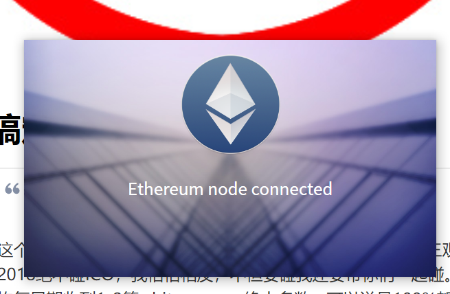
废话不说,首先去以太坊下载一个钱包。Ethereum Project
下载完了安装,你的界面应该是这样的:
官方的这个钱包bug非常多!经常打不开,而且和网络sync区块链的时候经常会有各种各样的问题……不过,如果你能侥幸安装成功并且同步成功。
恭喜你,你已经成功克服了你ICO道路上最大的技术难关,胜利在望,会所嫩模在向你招手!
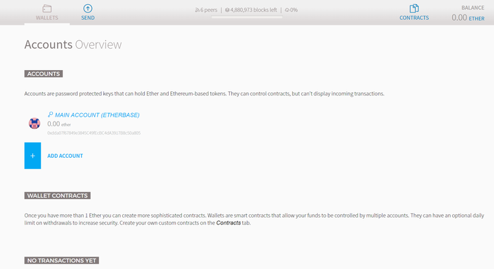
好,打开钱包,界面应该是下面这样:
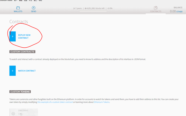
看到右上角那个“CONTRACTS"按钮了吗?轻轻点一下:
再点这个Deploy New Contract:
然后,打开这个网站:Create a cryptocurrency contract in Ethereum
不懂英文?没问题
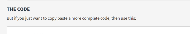
看不懂代码?无所谓
看到THE CODE了吗?
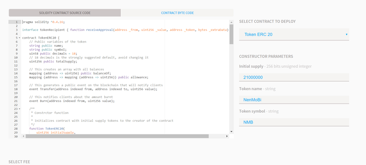
把下面的代码copy下来,然后粘贴到你的以太坊钱包里,再右边下来菜单里面选那个Token ERC 20 ,你会看到的界面大概是这个样子:
这个时候系统会让你输入三个参数:
Initial Supply:你要发行多少个币呢? 我填了2100万个,致敬比特币嘛!
Token Name:咱发行的币叫什么名字呢?我本来想叫刘易杰币……后来一想这太不中本聪了……不忘初衷,ICO骗钱为的就是会所嫩模,就叫嫩模币吧!
Token synbol:就是币的符号,比如比特币是BTC,以太坊是ETH,咱们嫩模币当然是NMB了!
然后下面有个蓝色的deploy,点了这个deploy,嫩模币就正式发布了————这里有个条件,就是钱包里要有少量的ETH,作为执行合约的Gas,大概是0.00几个ETH就够了,也就几美元到几十美元的事儿。
好了。
完成了。
如果你完成了如上所说的步骤的话,那么你成功的在这个世界上,基于以太坊网络,创造了一种新的加密货币————如果这破玩意儿能称为加密货币的话……
我大概解释一下啊这玩意儿是啥:以太坊网络和只能合约,支持一个use case就是用户可以通过以太坊来发行自己的"Token", Token是什么呢?
你可以理解为现实生活当中的“积分”,对,比如加油站洗车店会员卡积分,
楼下发廊Tony老师让你办的冲2000送1000的美发会员卡,奶茶点送你的盖满10个张送一杯的集戳卡,幼儿园老师给小朋友的小红花……
这一切的一切,都是可以在以太坊用很简单的只能合约代码搞成一个"token",然后Token可以通过以太坊网络转账, 转账的时候消耗少量的以太坊ETH做Gas。Token也不需要钱包——使用以太坊钱包就好,钱包地址也是以太坊的地址,钱包秘钥也是以太坊的秘钥,区块链用的就是以太坊的区块链……
说了这么多,就是想让你明白,Token这破玩意儿如此简单,发行如此容易,没有成本,完全是基于以太坊网络,没有任何自己的底层技术,基本上20分钟就能搞出来一个,供应量随便填。
我要说的是:现在有好多所谓的ICO,就是把这Token拿来当币卖……
如上所说创造出来的Token,跟比特币,以太坊,瑞波这些真的“加密货币"完全不是一个东西——我不是要给比特币以太坊这些数字货币站台——我一开始以为,要搞ICO,起码要像比特币那种,自己有区块链,有底层技术,分布账本,钱包,nodes都自己实现吧——虽然这也不是什么难事儿,毕竟都是开源的,但起码这还是有一定成本和壁垒的,结果,这帮骗钱骗疯了的,连这都不搞,直接像我上面发布嫩模币那样,利用小白韭菜们的无知,把Token拿来当成币卖……
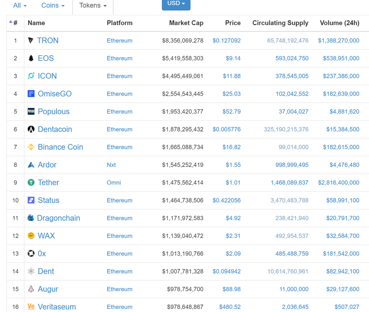
打开 All Tokens | CoinMarketCap看看哪些你以为和比特币,以太坊一样的加密货币,其实是和嫩模币NMB一样的Token呢?
有没有很眼熟啊?有没有很心慌啊?你看Platform,就是平台,多数都是以太坊平台,估值……50多亿美金?80多亿美金?
你们觉得嫩模币NMB估值应该多少啊?这么搞下去会不会币太多了,嫩模都不够用了啊……
好,现在币有了,接下来就是ICO难度最大的部分了:
写白皮书啊!
有没有发现现在白皮书天马星空,包罗万象,无所不能?为啥?本质上这玩意儿就是”积分“,能用的上”积分“的地方都能给套进去啊!机械制造,生物制药,航天科技,基因工程,物流运输,文化创作,阴阳五行,一带一路……反正你想怎么写怎么写,这部分就非常考验ICO团队的吹牛逼功力,白皮书写的不好,给观众的想象空间不够,基本可以判断,这个团队平时缺乏诈骗经验……
有了币,有了白皮书,就可以拿去忽悠人了,基本上就是说ICO前期,让对方给你打以太坊ETH,然后你给他发你的嫩模币NMB……他给你以太坊,你给他嫩模币,他给你ETH,你给他NMB……他的以太坊得是1000美金一个真金白银买的,你的NMB可是上面随手填出来的。过不过瘾?爽不爽?
这玩意儿,薄利多销,骗到50算50,骗到100算100,团队别露脸,白皮书上不写名,写名也别写自己名,找两个外国人做adviser,反正韭菜们也不会去验证。核心团队叫基金会,比如咱们负责操作嫩模币的基金会,可以起名叫NMB FOUNDATION。收到ETH直接变现分钱走人,或者另起炉灶,NMB ICO成功完成了,再搞下一个呗,市场需要细分,嫩模有的丑有的俏,针对丑嫩模搞一个丑嫩模币CNMB,俏嫩模的叫QNMB,或者叫嫩模2.0币NM2B,听上去就有互联网时代感……
区块链确实是个好技术,有很多潜力和空间,但究竟有没有好到颠覆世界,有没有好到随便发个tokn就能值十亿八亿的美金,有没有好到能让人打着”区块链“,”智能合约“,”加密货币“的幌子搞诈骗和非法集资能逃脱法律责任,有没有好到能让你买一个Token就赚个几百几千倍。大家自己判断。
*上面说的NMB合约我没deploy,所以你们不用找我要NMB了,不给你们。
**可以把这篇文章转给身边哪些被ICO忽悠的人,或者下次有人拿白皮书来忽悠你,你可以反杀他:你那个币不行,还是来投我的NMB吧!
【手把手教程】空投币怎么领取,以ShiBZilla为例
腾讯云 centos 门罗币 XMR 挖矿 教程 附代码 查看全部
3 天前
我本来是不想写这个的,昨天看了曹政的文章《不要试图挑战人性》,感触挺深的,曹大说他2018绝不碰ICO,我恰恰相反,不但要碰我还要带你们一起碰。ICO现在简直是太火了,我平均每星期收到1-2篇whitepaper,绝大多数,可以说是100%都是忽悠人的,我不当韭菜也会有别人被收割,莫不如我今天就给你们指条路——干嘛参与别人的ICO啊?你可以自己搞啊!
废话不说,首先去以太坊下载一个钱包。Ethereum Project
下载完了安装,你的界面应该是这样的:
官方的这个钱包bug非常多!经常打不开,而且和网络sync区块链的时候经常会有各种各样的问题……不过,如果你能侥幸安装成功并且同步成功。
恭喜你,你已经成功克服了你ICO道路上最大的技术难关,胜利在望,会所嫩模在向你招手!

好,打开钱包,界面应该是下面这样:
看到右上角那个“CONTRACTS"按钮了吗?轻轻点一下:
再点这个Deploy New Contract:
然后,打开这个网站:Create a cryptocurrency contract in Ethereum
不懂英文?没问题
看不懂代码?无所谓
看到THE CODE了吗?
把下面的代码copy下来,然后粘贴到你的以太坊钱包里,再右边下来菜单里面选那个Token ERC 20 ,你会看到的界面大概是这个样子:
这个时候系统会让你输入三个参数:
Initial Supply:你要发行多少个币呢? 我填了2100万个,致敬比特币嘛!
Token Name:咱发行的币叫什么名字呢?我本来想叫刘易杰币……后来一想这太不中本聪了……不忘初衷,ICO骗钱为的就是会所嫩模,就叫嫩模币吧!
Token synbol:就是币的符号,比如比特币是BTC,以太坊是ETH,咱们嫩模币当然是NMB了!
然后下面有个蓝色的deploy,点了这个deploy,嫩模币就正式发布了————这里有个条件,就是钱包里要有少量的ETH,作为执行合约的Gas,大概是0.00几个ETH就够了,也就几美元到几十美元的事儿。
好了。
完成了。
如果你完成了如上所说的步骤的话,那么你成功的在这个世界上,基于以太坊网络,创造了一种新的加密货币————如果这破玩意儿能称为加密货币的话……
我大概解释一下啊这玩意儿是啥:以太坊网络和只能合约,支持一个use case就是用户可以通过以太坊来发行自己的"Token", Token是什么呢?
你可以理解为现实生活当中的“积分”,对,比如加油站洗车店会员卡积分,
楼下发廊Tony老师让你办的冲2000送1000的美发会员卡,奶茶点送你的盖满10个张送一杯的集戳卡,幼儿园老师给小朋友的小红花……
这一切的一切,都是可以在以太坊用很简单的只能合约代码搞成一个"token",然后Token可以通过以太坊网络转账, 转账的时候消耗少量的以太坊ETH做Gas。Token也不需要钱包——使用以太坊钱包就好,钱包地址也是以太坊的地址,钱包秘钥也是以太坊的秘钥,区块链用的就是以太坊的区块链……
说了这么多,就是想让你明白,Token这破玩意儿如此简单,发行如此容易,没有成本,完全是基于以太坊网络,没有任何自己的底层技术,基本上20分钟就能搞出来一个,供应量随便填。
我要说的是:现在有好多所谓的ICO,就是把这Token拿来当币卖……
如上所说创造出来的Token,跟比特币,以太坊,瑞波这些真的“加密货币"完全不是一个东西——我不是要给比特币以太坊这些数字货币站台——我一开始以为,要搞ICO,起码要像比特币那种,自己有区块链,有底层技术,分布账本,钱包,nodes都自己实现吧——虽然这也不是什么难事儿,毕竟都是开源的,但起码这还是有一定成本和壁垒的,结果,这帮骗钱骗疯了的,连这都不搞,直接像我上面发布嫩模币那样,利用小白韭菜们的无知,把Token拿来当成币卖……
打开 All Tokens | CoinMarketCap看看哪些你以为和比特币,以太坊一样的加密货币,其实是和嫩模币NMB一样的Token呢?
有没有很眼熟啊?有没有很心慌啊?你看Platform,就是平台,多数都是以太坊平台,估值……50多亿美金?80多亿美金?
你们觉得嫩模币NMB估值应该多少啊?这么搞下去会不会币太多了,嫩模都不够用了啊……
好,现在币有了,接下来就是ICO难度最大的部分了:
写白皮书啊!
有没有发现现在白皮书天马星空,包罗万象,无所不能?为啥?本质上这玩意儿就是”积分“,能用的上”积分“的地方都能给套进去啊!机械制造,生物制药,航天科技,基因工程,物流运输,文化创作,阴阳五行,一带一路……反正你想怎么写怎么写,这部分就非常考验ICO团队的吹牛逼功力,白皮书写的不好,给观众的想象空间不够,基本可以判断,这个团队平时缺乏诈骗经验……
有了币,有了白皮书,就可以拿去忽悠人了,基本上就是说ICO前期,让对方给你打以太坊ETH,然后你给他发你的嫩模币NMB……他给你以太坊,你给他嫩模币,他给你ETH,你给他NMB……他的以太坊得是1000美金一个真金白银买的,你的NMB可是上面随手填出来的。过不过瘾?爽不爽?
这玩意儿,薄利多销,骗到50算50,骗到100算100,团队别露脸,白皮书上不写名,写名也别写自己名,找两个外国人做adviser,反正韭菜们也不会去验证。核心团队叫基金会,比如咱们负责操作嫩模币的基金会,可以起名叫NMB FOUNDATION。收到ETH直接变现分钱走人,或者另起炉灶,NMB ICO成功完成了,再搞下一个呗,市场需要细分,嫩模有的丑有的俏,针对丑嫩模搞一个丑嫩模币CNMB,俏嫩模的叫QNMB,或者叫嫩模2.0币NM2B,听上去就有互联网时代感……
区块链确实是个好技术,有很多潜力和空间,但究竟有没有好到颠覆世界,有没有好到随便发个tokn就能值十亿八亿的美金,有没有好到能让人打着”区块链“,”智能合约“,”加密货币“的幌子搞诈骗和非法集资能逃脱法律责任,有没有好到能让你买一个Token就赚个几百几千倍。大家自己判断。
*上面说的NMB合约我没deploy,所以你们不用找我要NMB了,不给你们。
**可以把这篇文章转给身边哪些被ICO忽悠的人,或者下次有人拿白皮书来忽悠你,你可以反杀他:你那个币不行,还是来投我的NMB吧!
【手把手教程】空投币怎么领取,以ShiBZilla为例
腾讯云 centos 门罗币 XMR 挖矿 教程 附代码
python模拟登录vexx.pro 获取你的总资产/币值和其他个人信息
python爬虫 • 李魔佛 发表了文章 • 0 个评论 • 4450 次浏览 • 2018-01-10 03:22
# -*-coding=utf-8-*-


import requests

session = requests.Session()

user = ''

password = ''


def getCode():

    headers = {

        'User-Agent': 'Mozilla/5.0 (Windows NT 6.1; Win64; x64) AppleWebKit/537.36 (KHTML, like Gecko) Chrome/62.0.3202.94 Safari/537.36'}

    url = 'http://vexx.pro/verify/code.html'

    s = session.get(url=url, headers=headers)


    with open('code.png', 'wb') as f:

        f.write(s.content)


    code = raw_input('input the code: ')

    print 'code is ', code


    login_url = 'http://vexx.pro/login/up_login.html'

    post_data = {

        'moble': user,

        'mobles': '+86',

        'password': password,

        'verify': code,

        'login_token': ''}


    login_s = session.post(url=login_url, headers=header, data=post_data)

    print login_s.status_code


    zzc_url = 'http://vexx.pro/ajax/check_zzc/'

    zzc_s = session.get(url=zzc_url, headers=headers)

    print zzc_s.text


def main():

    getCode()


if __name__ == '__main__':

    main()
把自己的用户名和密码填上去,中途输入一次验证码。
可以把session保存到本地,然后下一次就可以不用再输入密码。
后记: 经过几个月后,这个网站被证实是一个圈钱跑路的网站,目前已经无法正常登陆了。希望大家不要再上当了
原创地址:http://30daydo.com/article/263
转载请注明出处。 查看全部

# -*-coding=utf-8-*-
import requests
session = requests.Session()
user = ''
password = ''
def getCode():
headers = {
'User-Agent': 'Mozilla/5.0 (Windows NT 6.1; Win64; x64) AppleWebKit/537.36 (KHTML, like Gecko) Chrome/62.0.3202.94 Safari/537.36'}
url = 'http://vexx.pro/verify/code.html'
s = session.get(url=url, headers=headers)
with open('code.png', 'wb') as f:
f.write(s.content)
code = raw_input('input the code: ')
print 'code is ', code
login_url = 'http://vexx.pro/login/up_login.html'
post_data = {
'moble': user,
'mobles': '+86',
'password': password,
'verify': code,
'login_token': ''}
login_s = session.post(url=login_url, headers=header, data=post_data)
print login_s.status_code
zzc_url = 'http://vexx.pro/ajax/check_zzc/'
zzc_s = session.get(url=zzc_url, headers=headers)
print zzc_s.text
def main():
getCode()
if __name__ == '__main__':
main()
把自己的用户名和密码填上去,中途输入一次验证码。
可以把session保存到本地,然后下一次就可以不用再输入密码。
后记: 经过几个月后,这个网站被证实是一个圈钱跑路的网站,目前已经无法正常登陆了。希望大家不要再上当了
原创地址:http://30daydo.com/article/263
转载请注明出处。
python获取A股上市公司的盈利能力
量化交易-Ptrade-QMT • 李魔佛 发表了文章 • 0 个评论 • 7526 次浏览 • 2018-01-04 16:09
比如企业的盈利能力。
import tushare as ts

#获取2017年第3季度的盈利能力数据

ts.get_profit_data(2017,3)
返回的结果:
按年度、季度获取盈利能力数据,结果返回的数据属性说明如下:
code,代码
name,名称
roe,净资产收益率(%)
net_profit_ratio,净利率(%)
gross_profit_rate,毛利率(%)
net_profits,净利润(百万元) #这里的官网信息有误,单位应该是百万
esp,每股收益
business_income,营业收入(百万元)
bips,每股主营业务收入(元)
例如返回如下结果:
code name roe net_profit_ratio gross_profit_rate net_profits \
000717 韶钢松山 79.22 9.44 14.1042 1750.2624
600793 宜宾纸业 65.40 13.31 7.9084 100.6484
600306 商业城 63.19 18.55 17.8601 114.9175
000526 *ST紫学 61.03 2.78 31.1212 63.6477
600768 宁波富邦 57.83 14.95 2.7349 88.3171
原创,转载请注明:
http://30daydo.com/article/260
查看全部
比如企业的盈利能力。
import tushare as ts返回的结果:
#获取2017年第3季度的盈利能力数据
ts.get_profit_data(2017,3)
按年度、季度获取盈利能力数据,结果返回的数据属性说明如下:
code,代码
name,名称
roe,净资产收益率(%)
net_profit_ratio,净利率(%)
gross_profit_rate,毛利率(%)
net_profits,净利润(百万元) #这里的官网信息有误,单位应该是百万
esp,每股收益
business_income,营业收入(百万元)
bips,每股主营业务收入(元)
例如返回如下结果:
code name roe net_profit_ratio gross_profit_rate net_profits \
000717 韶钢松山 79.22 9.44 14.1042 1750.2624
600793 宜宾纸业 65.40 13.31 7.9084 100.6484
600306 商业城 63.19 18.55 17.8601 114.9175
000526 *ST紫学 61.03 2.78 31.1212 63.6477
600768 宁波富邦 57.83 14.95 2.7349 88.3171
原创,转载请注明:
http://30daydo.com/article/260
