30天尝试新事情

Price Momentum

股票 • 李魔佛发表了文章 • 0 个评论 • 3362 次浏览 • 2017-05-29 01:20 • 来自相关话题

Understanding Price Momentum

Today's stock market is more than just a place to buy and hold securities. Many investors prefer to move quickly in and out of the market. That's just one reason technical strategies, such as price momentum, have grown in popularity.

In this article, we're going to provide some insights into the investment strategy known as price momentum. We'll explain why some theorists believe this model offers investors a short-term profit opportunity. We'll also talk about the pros and cons of this approach, including the long-term opportunity that price momentum provides the market.

What is Price Momentum?

Additional Resources

Calculating Stock Prices
Capital Asset Pricing Model
Arbitrage Pricing Theory
Stock Beta and Volatility
Random Walk Theory Explained

The theory behind price momentum is relatively simple. Generally, we can talk about it in two ways; the first has to do with buying stocks:

Stocks that had relatively high returns over the past three to twelve months should return to investors above average returns over the next three to twelve months.

The theory also provides guidance on the right time to sell stocks:

Stocks that had relatively poor returns over the past three to twelve months should return to investors below average returns over the next three to twelve months.

This investment strategy was first theorized by Narasimhan Jegadeesh and Sheridan Titman in their publication "Returns to Buying Winners and Selling Losers: Implications for Stock Market Efficiency," which was published in The Journal of Finance back in March 1993.

Price Momentum Model

The model is based on the assumption the stock market is not completely efficient. This is something that most economists believe to be true. The two most practical explanations for the performance of this model include:

Investors are taking advantage of human behavior, including a "herding" mentality and / or an overreaction to news.
Investors employing a price momentum strategy are taking on additional risk; therefore, higher returns are required to compensate these investors for the risk they're assuming.

Within their study, Jegadeesh and Titman examined a large number of trading strategies. One of the conclusions from that study is stated below:

Buying past winners, and selling past losers, allowed investors to achieve above average returns over the period 1956 to 1989. In particular, stocks that were classified based on their prior 6-month performance, and held for 6 months realized an excess return of over 12% per year on average.

The Momentum Formula

Technical stock analysts understand the value this particular technique provides. They're constantly crunching numbers to see if patterns emerge. The actual formula for calculating price momentum is really quite simple, and takes the form:

M = CP - CPn

Where:

M = Momentum
CP = Closing price in the current period
CPn = Closing price N periods ago

For example, if a stock was trading at $35 per share six months ago, and is currently trading at $40 per share, then its six-month price momentum would be 40 minus 35 or 5.

Unfortunately, this formula is not normalized, and this makes it difficult to compare stocks selling at different price points. A stock experiencing a 1% price movement from $300 to $303 would have a momentum value of three. A second stock experiencing a 100% increase in price from $3 to $6 also has a momentum value of three.

Rate of Change Formula

One of the ways technical stock analysts can work around this problem is by calculating a rate of change value, which normalizes momentum:

RoC = (CP - CPn) / CPn

Where:

RoC = Rate of Change
CP = Closing price in the current period
CPn = Closing price N periods ago

Using the example above, the stock selling at $303 per share that was trading at $300 six months ago would have a Rate of Change of 3 / 300 or 1%, while the second stock would have a Rate of Change of 3 / 3 or 100%.

Momentum and Moving Averages

A second way that stock analysts use price momentum is in conjunction with moving averages. Here the technical analyst makes a series of price momentum calculations and plots these along with a moving average of the momentum.

For example, the plot might contain 28-day moving averages along with daily price momentum figures. Buy signals can be triggered when price momentum travels above its moving averages, and stays there for several trading days. Sell signals can be triggered when momentum travels below its moving average.

Contrarian Investing

As mentioned in the beginning of this article, this model tells investors they should buy past winners and sell past losers. Because this theory is based on past price performance, or historical market information, price momentum is a trading model that technical analysts would follow. Fundamental analysts believe that a stock is bought and sold based on its intrinsic value, including the company's potential to produce profits for its shareholders in the future.

Fortunately, fundamental analysts can also use price momentum to their advantage by adopting what is termed a contrarian investing strategy. Contrarian investors take the opposite approach that a theory advocates. For example, a fundamental analyst might conclude:

A stock that has been rising may now be overvalued, while a stock that has been falling may be undervalued.

One could argue the further a stock moves from its true market value, the greater the opportunity for profits. By tracking price momentum, and using this as a screening tool, fundamental analysts can then assess if a stock is truly undervalued or overvalued by studying the company's long-term financial health and earnings power.

About the Author - Understanding Price Momentum (Last Reviewed on November 22, 2016)

http://30daydo.com/article/203
查看全部

Understanding Price Momentum

Today's stock market is more than just a place to buy and hold securities. Many investors prefer to move quickly in and out of the market. That's just one reason technical strategies, such as price momentum, have grown in popularity.

In this article, we're going to provide some insights into the investment strategy known as price momentum. We'll explain why some theorists believe this model offers investors a short-term profit opportunity. We'll also talk about the pros and cons of this approach, including the long-term opportunity that price momentum provides the market.

What is Price Momentum?

Additional Resources

Calculating Stock Prices
Capital Asset Pricing Model
Arbitrage Pricing Theory
Stock Beta and Volatility
Random Walk Theory Explained

The theory behind price momentum is relatively simple. Generally, we can talk about it in two ways; the first has to do with buying stocks:

Stocks that had relatively high returns over the past three to twelve months should return to investors above average returns over the next three to twelve months.

The theory also provides guidance on the right time to sell stocks:

Stocks that had relatively poor returns over the past three to twelve months should return to investors below average returns over the next three to twelve months.

This investment strategy was first theorized by Narasimhan Jegadeesh and Sheridan Titman in their publication "Returns to Buying Winners and Selling Losers: Implications for Stock Market Efficiency," which was published in The Journal of Finance back in March 1993.

Price Momentum Model

The model is based on the assumption the stock market is not completely efficient. This is something that most economists believe to be true. The two most practical explanations for the performance of this model include:

Investors are taking advantage of human behavior, including a "herding" mentality and / or an overreaction to news.
Investors employing a price momentum strategy are taking on additional risk; therefore, higher returns are required to compensate these investors for the risk they're assuming.

Within their study, Jegadeesh and Titman examined a large number of trading strategies. One of the conclusions from that study is stated below:

Buying past winners, and selling past losers, allowed investors to achieve above average returns over the period 1956 to 1989. In particular, stocks that were classified based on their prior 6-month performance, and held for 6 months realized an excess return of over 12% per year on average.

The Momentum Formula

Technical stock analysts understand the value this particular technique provides. They're constantly crunching numbers to see if patterns emerge. The actual formula for calculating price momentum is really quite simple, and takes the form:

M = CP - CPn

Where:

M = Momentum
CP = Closing price in the current period
CPn = Closing price N periods ago

For example, if a stock was trading at $35 per share six months ago, and is currently trading at $40 per share, then its six-month price momentum would be 40 minus 35 or 5.

Unfortunately, this formula is not normalized, and this makes it difficult to compare stocks selling at different price points. A stock experiencing a 1% price movement from $300 to $303 would have a momentum value of three. A second stock experiencing a 100% increase in price from $3 to $6 also has a momentum value of three.

Rate of Change Formula

One of the ways technical stock analysts can work around this problem is by calculating a rate of change value, which normalizes momentum:

RoC = (CP - CPn) / CPn

Where:

RoC = Rate of Change
CP = Closing price in the current period
CPn = Closing price N periods ago

Using the example above, the stock selling at $303 per share that was trading at $300 six months ago would have a Rate of Change of 3 / 300 or 1%, while the second stock would have a Rate of Change of 3 / 3 or 100%.

Momentum and Moving Averages

A second way that stock analysts use price momentum is in conjunction with moving averages. Here the technical analyst makes a series of price momentum calculations and plots these along with a moving average of the momentum.

For example, the plot might contain 28-day moving averages along with daily price momentum figures. Buy signals can be triggered when price momentum travels above its moving averages, and stays there for several trading days. Sell signals can be triggered when momentum travels below its moving average.

Contrarian Investing

As mentioned in the beginning of this article, this model tells investors they should buy past winners and sell past losers. Because this theory is based on past price performance, or historical market information, price momentum is a trading model that technical analysts would follow. Fundamental analysts believe that a stock is bought and sold based on its intrinsic value, including the company's potential to produce profits for its shareholders in the future.

Fortunately, fundamental analysts can also use price momentum to their advantage by adopting what is termed a contrarian investing strategy. Contrarian investors take the opposite approach that a theory advocates. For example, a fundamental analyst might conclude:

A stock that has been rising may now be overvalued, while a stock that has been falling may be undervalued.

One could argue the further a stock moves from its true market value, the greater the opportunity for profits. By tracking price momentum, and using this as a screening tool, fundamental analysts can then assess if a stock is truly undervalued or overvalued by studying the company's long-term financial health and earnings power.

About the Author - Understanding Price Momentum (Last Reviewed on November 22, 2016)

http://30daydo.com/article/203

能否改变贫穷?

每日总结 • 李魔佛发表了文章 • 0 个评论 • 3008 次浏览 • 2017-05-29 01:17 • 来自相关话题

这是我的博士同事，Naphet，10月20日下午3点，他正式打出了他的博士论文，完成了四年的博士生涯。

Naphet 来自津巴布韦，世界上最混乱的国家之一（也许没有之一）。他没有谈他的童年，但我知道那一定不是我可以相比的。他从家乡出来后，成功地申请到了我们学校的 PhD，并且获得了英国国籍。这中间的努力，真的是我难以想象的。我至今深深记得，他去参加他的博士论文答辩的那天，抱着一本300多页厚厚的博士论文，像抱着一个婴儿那么珍惜。他的论文做定量的，主要工具是spss 程序，我曾经问过他从哪里学的 spss，他和我说，他在网上自学的。在读博的三年时间里，他就通过看 Youtube 的在线视频来从0开始学习 spss，如今，他的论文里充斥着各种精致的公式，而我的论文相比之下是如此的苍白无力。但他的论文还是没有通过答辩，因为我们学校新来的一个女老师质疑了他的方法，他很愤怒，因为他不理解为什么自己学校的老师竟然不支持他，但他没有气馁，而是继续每天早出晚归地来研究室修改论文。

他是有两个孩子的单亲爸爸。女儿已经上了高中，儿子才几个月大。他白天要在家里带孩子，晚上到火车站开出租车补贴学费和家用，挣来的钱还要寄回津巴布韦老家。因此他白天在家里通过远程桌面连接学校电脑学习，只有在晚上五点以后，他的女儿放学回来能照顾自己的弟弟，以及出租下班的时候才能来研究室学习。他周末的时候从来不回家，睡在出租车里，这样能多挣钱。而他一旦坐下，就会一动不动地全神贯注地开始工作。我有时候都很奇怪他从哪里来的精力，能够一边打工一边学习，并且能够如此专注。每每午夜十二点半，我离开研究室，而他仍然坐在电脑屏幕面前，专心调整着他公式的参数。

Naphet 的女儿非常优秀，她6岁的时候来到他身边。他充满自豪地同我分享了她女儿在 BBC 演讲比赛中获胜的演讲，并且告诉我她是英国青少年议会的议员，教区领袖，学校青少年协会的领导。“她的生活非常自律，比我更加自律，我从来没见过一个哪个17岁的孩子能够像她那么生活。”他对我说。在他女儿十五岁参加的那场演讲中，她把英语称之为杀手，并且分析了外国移民在英文环境中面对的语言困境。“我没有写一个字给她，都是她自己写的。我把这个视频用到了我的课程'社会学的想象力'中，这是一个可以作为博士论文的课题。”Naphet 非常自豪地对我说。我真的很震惊一个十五岁的女孩能够对环境有如此的敏感性。我提醒 Naphet 不要让她过于骄傲，他和我说：“我从来不夸奖她，我只是告诉她需要面对的挑战。她能够完成每一项挑战。”

他曾和我分享了他求职失败的经历，原因竟然是他过于优秀。三年博士期间，他获得了多个教师资格证书，比他的面试官还要优秀。结果可想而知，他精心准备的演讲反而害了他，实在是十分荒谬。但他没有气馁，他和我说：“我目前需要做的就是尽快博士毕业，好让自己有更多的自由去寻找更好的机会。”他的教学经验之丰富，远远超过了他的同辈，连他的面试官也只能嫉妒地说：“你实在是走的太快了。”我问他关于论文引用的问题，他却反过来向我求教我使用的引用软件，等我介绍完之后他掏出本子认真的记录着：“这个软件很好，我以后也要让我女儿试试。我现在就在为她准备大学需要面临的一切。”那一刻，我真的感觉到为什么人们说机会都是留给有准备的人。什么样的人是优秀的人？自强，自律，虚心，不骄不躁，永远充满信心，这样的父亲有这样的女儿，一点也不奇怪。

人在海外，社交圈很小，因此他给我的触动反倒更大。我第一次认真思考了何为一个有担当的男人。他没有钱，所以出去工作，他没有知识，所以上网自学。他面对着所有的不公正，却充满了自信的微笑。他对我说：“我要尽快完成我的博士，向我女儿证明我可以做到这一切。”是的，他一定可以的，我一点都不怀疑。反观我自己，在每一点上都放佛要被压榨出一个大大的“小”字来，我连对比的勇气都没有。他那岩石一般英朗的笑容背后有多少辛酸，多少委屈，我无法猜测，但我看到的是，他如同钟表一样准时的每天来到研究室，坐下，学习，创造着属于他和他女儿的未来。

他在论文的致谢部分写着：“献给我的母亲和我的四个兄弟，献给我过世的爸爸和五个叔叔。”

“我已经很多年没见过我母亲了。”他看着我读完了致谢之后说。

“你是怎么走过这一切的呢？”我问。

“压力。生活挤压着你，你只有前进。我所获得的一切都是靠我自己的双手得来的。”

他，是他们五兄弟中唯一走出来的。

很多时候，Naphet 这样的人是学不来的，但我想，他本身也许就是一个答案，在我们陷入迷茫和懦弱时，在我们给自己的人生拼命找借口时，带来一个声音：

贫穷不能改变吗？

能。

转至知乎：
https://www.zhihu.com/question/28098030/answer/68722565
查看全部

这是我的博士同事，Naphet，10月20日下午3点，他正式打出了他的博士论文，完成了四年的博士生涯。

Naphet 来自津巴布韦，世界上最混乱的国家之一（也许没有之一）。他没有谈他的童年，但我知道那一定不是我可以相比的。他从家乡出来后，成功地申请到了我们学校的 PhD，并且获得了英国国籍。这中间的努力，真的是我难以想象的。我至今深深记得，他去参加他的博士论文答辩的那天，抱着一本300多页厚厚的博士论文，像抱着一个婴儿那么珍惜。他的论文做定量的，主要工具是spss 程序，我曾经问过他从哪里学的 spss，他和我说，他在网上自学的。在读博的三年时间里，他就通过看 Youtube 的在线视频来从0开始学习 spss，如今，他的论文里充斥着各种精致的公式，而我的论文相比之下是如此的苍白无力。但他的论文还是没有通过答辩，因为我们学校新来的一个女老师质疑了他的方法，他很愤怒，因为他不理解为什么自己学校的老师竟然不支持他，但他没有气馁，而是继续每天早出晚归地来研究室修改论文。

他是有两个孩子的单亲爸爸。女儿已经上了高中，儿子才几个月大。他白天要在家里带孩子，晚上到火车站开出租车补贴学费和家用，挣来的钱还要寄回津巴布韦老家。因此他白天在家里通过远程桌面连接学校电脑学习，只有在晚上五点以后，他的女儿放学回来能照顾自己的弟弟，以及出租下班的时候才能来研究室学习。他周末的时候从来不回家，睡在出租车里，这样能多挣钱。而他一旦坐下，就会一动不动地全神贯注地开始工作。我有时候都很奇怪他从哪里来的精力，能够一边打工一边学习，并且能够如此专注。每每午夜十二点半，我离开研究室，而他仍然坐在电脑屏幕面前，专心调整着他公式的参数。

Naphet 的女儿非常优秀，她6岁的时候来到他身边。他充满自豪地同我分享了她女儿在 BBC 演讲比赛中获胜的演讲，并且告诉我她是英国青少年议会的议员，教区领袖，学校青少年协会的领导。“她的生活非常自律，比我更加自律，我从来没见过一个哪个17岁的孩子能够像她那么生活。”他对我说。在他女儿十五岁参加的那场演讲中，她把英语称之为杀手，并且分析了外国移民在英文环境中面对的语言困境。“我没有写一个字给她，都是她自己写的。我把这个视频用到了我的课程'社会学的想象力'中，这是一个可以作为博士论文的课题。”Naphet 非常自豪地对我说。我真的很震惊一个十五岁的女孩能够对环境有如此的敏感性。我提醒 Naphet 不要让她过于骄傲，他和我说：“我从来不夸奖她，我只是告诉她需要面对的挑战。她能够完成每一项挑战。”

他曾和我分享了他求职失败的经历，原因竟然是他过于优秀。三年博士期间，他获得了多个教师资格证书，比他的面试官还要优秀。结果可想而知，他精心准备的演讲反而害了他，实在是十分荒谬。但他没有气馁，他和我说：“我目前需要做的就是尽快博士毕业，好让自己有更多的自由去寻找更好的机会。”他的教学经验之丰富，远远超过了他的同辈，连他的面试官也只能嫉妒地说：“你实在是走的太快了。”我问他关于论文引用的问题，他却反过来向我求教我使用的引用软件，等我介绍完之后他掏出本子认真的记录着：“这个软件很好，我以后也要让我女儿试试。我现在就在为她准备大学需要面临的一切。”那一刻，我真的感觉到为什么人们说机会都是留给有准备的人。什么样的人是优秀的人？自强，自律，虚心，不骄不躁，永远充满信心，这样的父亲有这样的女儿，一点也不奇怪。

人在海外，社交圈很小，因此他给我的触动反倒更大。我第一次认真思考了何为一个有担当的男人。他没有钱，所以出去工作，他没有知识，所以上网自学。他面对着所有的不公正，却充满了自信的微笑。他对我说：“我要尽快完成我的博士，向我女儿证明我可以做到这一切。”是的，他一定可以的，我一点都不怀疑。反观我自己，在每一点上都放佛要被压榨出一个大大的“小”字来，我连对比的勇气都没有。他那岩石一般英朗的笑容背后有多少辛酸，多少委屈，我无法猜测，但我看到的是，他如同钟表一样准时的每天来到研究室，坐下，学习，创造着属于他和他女儿的未来。

他在论文的致谢部分写着：“献给我的母亲和我的四个兄弟，献给我过世的爸爸和五个叔叔。”

“我已经很多年没见过我母亲了。”他看着我读完了致谢之后说。

“你是怎么走过这一切的呢？”我问。

“压力。生活挤压着你，你只有前进。我所获得的一切都是靠我自己的双手得来的。”

他，是他们五兄弟中唯一走出来的。

很多时候，Naphet 这样的人是学不来的，但我想，他本身也许就是一个答案，在我们陷入迷茫和懦弱时，在我们给自己的人生拼命找借口时，带来一个声音：

贫穷不能改变吗？

能。

转至知乎：
https://www.zhihu.com/question/28098030/answer/68722565

TA-Lib MA_Type

股票 • 李魔佛发表了文章 • 0 个评论 • 17709 次浏览 • 2017-05-29 00:43 • 来自相关话题

在TA-Lib中有一个参数的类型是MA_Type，谷歌了一下，把内容贴出来。

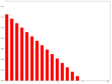
主要就是使用不一样的加权方式对数据进行处理。import talib
from talib import MA_Type

MA_Type: 0=SMA, 1=EMA, 2=WMA, 3=DEMA, 4=TEMA, 5=TRIMA, 6=KAMA, 7=MAMA, 8=T3 (Default=SMA)

移动平均（英语：moving average，MA），又称“移动平均线”简称均线，是技术分析中一种分析时间序列数据的工具。最常见的是利用股价、回报或交易量等变数计算出移动平均。
移动平均可抚平短期波动，反映出长期趋势或周期。数学上，移动平均可视为一种卷积。

简单移动平均（英语：simple moving average，SMA）是某变数之前n个数值的未作加权算术平均。例如，收市价的10日简单移动平均指之前10日收市价的平均数。：

当计算连续的数值，一个新的数值加入，同时一个旧数值剔出，所以无需每次都重新逐个数值加起来。
在技术分析中，不同的市场对常用天数（n值）有不同的需求，例如：某些市场普遍的n值为10日、40日、200日；有些则是5日、10日、20日、60日、120日、240日，视乎分析时期长短而定。投资者冀从移动平均线的图表中分辨出支持位或阻力位。

加权移动平均（英语：weighted moving average，WMA）指计算平均值时将个别数据乘以不同数值，在技术分析中，n日WMA的最近期一个数值乘以n、次近的乘以n-1，如此类推，一直到0：

指数移动平均（英语：exponential moving average，EMA或EWMA）是以指数式递减加权的移动平均。各数值的加权影响力随时间而指数式递减，越近期的数据加权影响力越重，但较旧的数据也给予一定的加权值

WMA EMA

使用下面的代码实现不一样的MA
#MA_Type: 0=SMA, 1=EMA, 2=WMA, 3=DEMA, 4=TEMA, 5=TRIMA, 6=KAMA, 7=MAMA, 8=T3 (Default=SMA)
df=ts.get_k_data('300580',start='2017-01-12',end='2017-05-26')
closed=df['close'].values
sma=talib.MA(closed,timeperiod=10,matype=0)
ema=talib.MA(closed,timeperiod=10,matype=1)
wma=talib.MA(closed,timeperiod=10,matype=2)
dema=talib.MA(closed,timeperiod=10,matype=3)
tema=talib.MA(closed,timeperiod=10,matype=4)
trima=talib.MA(closed,timeperiod=10,matype=5)
kma=talib.MA(closed,timeperiod=10,matype=6)
mama=talib.MA(closed,timeperiod=10,matype=7)
t3=talib.MA(closed,timeperiod=10,matype=8)
#ouput=talib.MA(closed,timeperiod=5,matype=0)
print closed
plt.ylim([0,40])
plt.plot(sma)
plt.plot(ema)
plt.plot(wma)
plt.plot(dema)
plt.plot(tema)
plt.plot(trima)
plt.plot(kma)
plt.plot(mama)
plt.plot(t3)
plt.grid()
plt.show()
生成的图像如下：

http://30daydo.com/article/201
转载请注明出处查看全部

在TA-Lib中有一个参数的类型是MA_Type，谷歌了一下，把内容贴出来。

主要就是使用不一样的加权方式对数据进行处理。

import talib

from talib import MA_Type



MA_Type: 0=SMA, 1=EMA, 2=WMA, 3=DEMA, 4=TEMA, 5=TRIMA, 6=KAMA, 7=MAMA, 8=T3 (Default=SMA)

移动平均（英语：moving average，MA），又称“移动平均线”简称均线，是技术分析中一种分析时间序列数据的工具。最常见的是利用股价、回报或交易量等变数计算出移动平均。
移动平均可抚平短期波动，反映出长期趋势或周期。数学上，移动平均可视为一种卷积。

简单移动平均（英语：simple moving average，SMA）是某变数之前n个数值的未作加权算术平均。例如，收市价的10日简单移动平均指之前10日收市价的平均数。：

当计算连续的数值，一个新的数值加入，同时一个旧数值剔出，所以无需每次都重新逐个数值加起来。
在技术分析中，不同的市场对常用天数（n值）有不同的需求，例如：某些市场普遍的n值为10日、40日、200日；有些则是5日、10日、20日、60日、120日、240日，视乎分析时期长短而定。投资者冀从移动平均线的图表中分辨出支持位或阻力位。

加权移动平均（英语：weighted moving average，WMA）指计算平均值时将个别数据乘以不同数值，在技术分析中，n日WMA的最近期一个数值乘以n、次近的乘以n-1，如此类推，一直到0：

指数移动平均（英语：exponential moving average，EMA或EWMA）是以指数式递减加权的移动平均。各数值的加权影响力随时间而指数式递减，越近期的数据加权影响力越重，但较旧的数据也给予一定的加权值

WMA EMA

使用下面的代码实现不一样的MA

    #MA_Type: 0=SMA, 1=EMA, 2=WMA, 3=DEMA, 4=TEMA, 5=TRIMA, 6=KAMA, 7=MAMA, 8=T3 (Default=SMA)

    df=ts.get_k_data('300580',start='2017-01-12',end='2017-05-26')

    closed=df['close'].values

    sma=talib.MA(closed,timeperiod=10,matype=0)

    ema=talib.MA(closed,timeperiod=10,matype=1)

    wma=talib.MA(closed,timeperiod=10,matype=2)

    dema=talib.MA(closed,timeperiod=10,matype=3)

    tema=talib.MA(closed,timeperiod=10,matype=4)

    trima=talib.MA(closed,timeperiod=10,matype=5)

    kma=talib.MA(closed,timeperiod=10,matype=6)

    mama=talib.MA(closed,timeperiod=10,matype=7)

    t3=talib.MA(closed,timeperiod=10,matype=8)

    #ouput=talib.MA(closed,timeperiod=5,matype=0)

    print closed

    plt.ylim([0,40])

    plt.plot(sma)

    plt.plot(ema)

    plt.plot(wma)

    plt.plot(dema)

    plt.plot(tema)

    plt.plot(trima)

    plt.plot(kma)

    plt.plot(mama)

    plt.plot(t3)

    plt.grid()

    plt.show()

生成的图像如下：

http://30daydo.com/article/201
转载请注明出处

TA-Lib 量化交易代码实例 <二> 获取布林线的上轨，中轨，下轨的数据

量化交易-Ptrade-QMT • 李魔佛发表了文章 • 0 个评论 • 24455 次浏览 • 2017-05-28 23:08 • 来自相关话题

BOLL指标的原理
BOLL指标是美国股市分析家约翰·布林根据统计学中的标准差原理设计出来的一种非常简单实用的技术分析指标。一般而言，股价的运动总是围绕某一价值中枢（如均线、成本线等）在一定的范围内变动，布林线指标指标正是在上述条件的基础上，引进了“股价通道”的概念，其认为股价通道的宽窄随着股价波动幅度的大小而变化，而且股价通道又具有变异性，它会随着股价的变化而自动调整。正是由于它具有灵活性、直观性和趋势性的特点，BOLL指标渐渐成为投资者广为应用的市场上热门指标。
在众多技术分析指标中，BOLL指标属于比较特殊的一类指标。绝大多数技术分析指标都是通过数量的方法构造出来的，它们本身不依赖趋势分析和形态分析，而BOLL指标却股价的形态和趋势有着密不可分的联系。BOLL指标中的“股价通道”概念正是股价趋势理论的直观表现形式。BOLL是利用“股价通道”来显示股价的各种价位，当股价波动很小，处于盘整时，股价通道就会变窄，这可能预示着股价的波动处于暂时的平静期；当股价波动超出狭窄的股价通道的上轨时，预示着股价的异常激烈的向上波动即将开始；当股价波动超出狭窄的股价通道的下轨时，同样也预示着股价的异常激烈的向下波动将开始。
投资者常常会遇到两种最常见的交易陷阱，一是买低陷阱，投资者在所谓的低位买进之后，股价不仅没有止跌反而不断下跌；二是卖高陷阱，股票在所谓的高点卖出后，股价却一路上涨。布林线特别运用了爱因斯坦的相对论，认为各类市场间都是互动的，市场内和市场间的各种变化都是相对性的，是不存在绝对性的，股价的高低是相对的，股价在上轨线以上或在下轨线以下只反映该股股价相对较高或较低，投资者作出投资判断前还须综合参考其他技术指标，包括价量配合，心理类指标，类比类指标，市场间的关联数据等。
总之，BOLL指标中的股价通道对预测未来行情的走势起着重要的参考作用，它也是布林线指标所特有的分析手段。
[编辑]
BOLL指标的计算方法
在所有的指标计算中，BOLL指标的计算方法是最复杂的之一，其中引进了统计学中的标准差概念，涉及到中轨线（MB）、上轨线（UP）和下轨线（DN）的计算。另外，和其他指标的计算一样，由于选用的计算周期的不同，BOLL指标也包括日BOLL指标、周BOLL指标、月BOLL指标年BOLL指标以及分钟BOLL指标等各种类型。经常被用于股市研判的是日BOLL指标和周BOLL指标。虽然它们的计算时的取值有所不同，但基本的计算方法一样。以日BOLL指标计算为例，其计算方法如下：
1、日BOLL指标的计算公式
中轨线=N日的移动平均线
上轨线=中轨线＋两倍的标准差
下轨线=中轨线－两倍的标准差
2、日BOLL指标的计算过程
1）计算MA
MA=N日内的收盘价之和÷N2）计算标准差MD
MD=平方根N日的（C－MA）的两次方之和除以N3）计算MB、UP、DN线
MB=（N－1）日的MA
UP=MB＋2×MD
DN=MB－2×MD在股市分析软件中，BOLL指标一共由四条线组成，即上轨线UP 、中轨线MB、下轨线DN和价格线。其中上轨线UP是UP数值的连线，用黄色线表示；中轨线MB是MB数值的连线，用白色线表示；下轨线DN是DN数值的连线，用紫色线表示；价格线是以美国线表示，颜色为浅蓝色。和其他技术指标一样，在实战中，投资者不需要进行BOLL指标的计算，主要是了解BOLL的计算方法和过程，以便更加深入地掌握BOLL指标的实质，为运用指标打下基础。

#通过tushare获取股票信息
df=ts.get_k_data('300580',start='2017-01-12',end='2017-05-26')
#提取收盘价
closed=df['close'].values

upper,middle,lower=talib.BBANDS(closed,matype=talib.MA_Type.T3)

print upper,middle,lower
plt.plot(upper)
plt.plot(middle)
plt.plot(lower)
plt.grid()
plt.show()
diff1=upper-middle
diff2=middle-lower
print diff1
print diff2

最后那里可以看到diff1和diff2是一样的。验证了布林线的定义ma+2d，m-2d。查看全部

BOLL指标的原理
BOLL指标是美国股市分析家约翰·布林根据统计学中的标准差原理设计出来的一种非常简单实用的技术分析指标。一般而言，股价的运动总是围绕某一价值中枢（如均线、成本线等）在一定的范围内变动，布林线指标指标正是在上述条件的基础上，引进了“股价通道”的概念，其认为股价通道的宽窄随着股价波动幅度的大小而变化，而且股价通道又具有变异性，它会随着股价的变化而自动调整。正是由于它具有灵活性、直观性和趋势性的特点，BOLL指标渐渐成为投资者广为应用的市场上热门指标。
在众多技术分析指标中，BOLL指标属于比较特殊的一类指标。绝大多数技术分析指标都是通过数量的方法构造出来的，它们本身不依赖趋势分析和形态分析，而BOLL指标却股价的形态和趋势有着密不可分的联系。BOLL指标中的“股价通道”概念正是股价趋势理论的直观表现形式。BOLL是利用“股价通道”来显示股价的各种价位，当股价波动很小，处于盘整时，股价通道就会变窄，这可能预示着股价的波动处于暂时的平静期；当股价波动超出狭窄的股价通道的上轨时，预示着股价的异常激烈的向上波动即将开始；当股价波动超出狭窄的股价通道的下轨时，同样也预示着股价的异常激烈的向下波动将开始。
投资者常常会遇到两种最常见的交易陷阱，一是买低陷阱，投资者在所谓的低位买进之后，股价不仅没有止跌反而不断下跌；二是卖高陷阱，股票在所谓的高点卖出后，股价却一路上涨。布林线特别运用了爱因斯坦的相对论，认为各类市场间都是互动的，市场内和市场间的各种变化都是相对性的，是不存在绝对性的，股价的高低是相对的，股价在上轨线以上或在下轨线以下只反映该股股价相对较高或较低，投资者作出投资判断前还须综合参考其他技术指标，包括价量配合，心理类指标，类比类指标，市场间的关联数据等。
总之，BOLL指标中的股价通道对预测未来行情的走势起着重要的参考作用，它也是布林线指标所特有的分析手段。
[编辑]
BOLL指标的计算方法
在所有的指标计算中，BOLL指标的计算方法是最复杂的之一，其中引进了统计学中的标准差概念，涉及到中轨线（MB）、上轨线（UP）和下轨线（DN）的计算。另外，和其他指标的计算一样，由于选用的计算周期的不同，BOLL指标也包括日BOLL指标、周BOLL指标、月BOLL指标年BOLL指标以及分钟BOLL指标等各种类型。经常被用于股市研判的是日BOLL指标和周BOLL指标。虽然它们的计算时的取值有所不同，但基本的计算方法一样。以日BOLL指标计算为例，其计算方法如下：
1、日BOLL指标的计算公式
中轨线=N日的移动平均线
上轨线=中轨线＋两倍的标准差
下轨线=中轨线－两倍的标准差
2、日BOLL指标的计算过程
1）计算MA
MA=N日内的收盘价之和÷N2）计算标准差MD
MD=平方根N日的（C－MA）的两次方之和除以N3）计算MB、UP、DN线
MB=（N－1）日的MA
UP=MB＋2×MD
DN=MB－2×MD在股市分析软件中，BOLL指标一共由四条线组成，即上轨线UP 、中轨线MB、下轨线DN和价格线。其中上轨线UP是UP数值的连线，用黄色线表示；中轨线MB是MB数值的连线，用白色线表示；下轨线DN是DN数值的连线，用紫色线表示；价格线是以美国线表示，颜色为浅蓝色。和其他技术指标一样，在实战中，投资者不需要进行BOLL指标的计算，主要是了解BOLL的计算方法和过程，以便更加深入地掌握BOLL指标的实质，为运用指标打下基础。

    #通过tushare获取股票信息

    df=ts.get_k_data('300580',start='2017-01-12',end='2017-05-26')

    #提取收盘价

    closed=df['close'].values

    

    upper,middle,lower=talib.BBANDS(closed,matype=talib.MA_Type.T3)

    

    print upper,middle,lower

    plt.plot(upper)

    plt.plot(middle)

    plt.plot(lower)

    plt.grid()

    plt.show()

    diff1=upper-middle

    diff2=middle-lower

    print diff1

    print diff2

最后那里可以看到diff1和diff2是一样的。验证了布林线的定义ma+2d，m-2d。

quantdigger 量化交易入门代码示例

量化交易-Ptrade-QMT • 李魔佛发表了文章 • 1 个评论 • 4552 次浏览 • 2017-05-28 21:39 • 来自相关话题

第五天

《》
待更新

TA-Lib 量化交易代码实例 <一> 获取5日，10日，20日均线数据

量化交易-Ptrade-QMT • 李魔佛发表了文章 • 0 个评论 • 24030 次浏览 • 2017-05-28 21:37 • 来自相关话题

第一节

安装教程在前面内容已经介绍过了，对于新手也是有点障碍，可以参照前面的文章进行一步一步操作。 http://30daydo.com/article/195 #通过tushare获取股票信息
df=ts.get_k_data('300580',start='2017-01-12',end='2017-05-26')
#提取收盘价
closed=df['close'].values
#获取均线的数据，通过timeperiod参数来分别获取 5,10,20 日均线的数据。
ma5=talib.SMA(closed,timeperiod=5)
ma10=talib.SMA(closed,timeperiod=10)
ma20=talib.SMA(closed,timeperiod=20)

#打印出来每一个数据
print closed
print ma5
print ma10
print ma20

#通过plog函数可以很方便的绘制出每一条均线
plt.plot(closed)
plt.plot(ma5)
plt.plot(ma10)
plt.plot(ma20)
#添加网格，可有可无，只是让图像好看点
plt.grid()
#记得加这一句，不然不会显示图像
plt.show()
上面第一句使用tushare获取股票的数据，如果不知道怎么操作的，可以在这里参考，同样是入门的教程。
http://30daydo.com/article/13

运行上面的代码后，可以得到下面的曲线：

你们可以去对比一下贝斯特的收盘价，5日，10日，20日均线。是不是一样的？
就这样我们就完成了均线的获取。是不是很简单？

查看全部

第一节

安装教程在前面内容已经介绍过了，对于新手也是有点障碍，可以参照前面的文章进行一步一步操作。 http://30daydo.com/article/195

    #通过tushare获取股票信息

    df=ts.get_k_data('300580',start='2017-01-12',end='2017-05-26')

    #提取收盘价

    closed=df['close'].values

    #获取均线的数据，通过timeperiod参数来分别获取 5,10,20 日均线的数据。

    ma5=talib.SMA(closed,timeperiod=5)

    ma10=talib.SMA(closed,timeperiod=10)

    ma20=talib.SMA(closed,timeperiod=20)



    #打印出来每一个数据

    print closed

    print ma5

    print ma10

    print ma20



    #通过plog函数可以很方便的绘制出每一条均线

    plt.plot(closed)

    plt.plot(ma5)

    plt.plot(ma10)

    plt.plot(ma20)

    #添加网格，可有可无，只是让图像好看点

    plt.grid()

    #记得加这一句，不然不会显示图像

    plt.show()

上面第一句使用tushare获取股票的数据，如果不知道怎么操作的，可以在这里参考，同样是入门的教程。
http://30daydo.com/article/13

运行上面的代码后，可以得到下面的曲线：

你们可以去对比一下贝斯特的收盘价，5日，10日，20日均线。是不是一样的？
就这样我们就完成了均线的获取。是不是很简单？

ImportError: No module named _tkinter

python • 李魔佛发表了文章 • 0 个评论 • 6526 次浏览 • 2017-05-28 21:33 • 来自相关话题

ImportError: No module named _tkinter, please install the python-tk package ubuntu运行tkinter错误

这是由于Python的版本没有包含tkinter的模块，只需要把tk的package安装就可以了。一般在Linux才出现，windows版本一般已经包含了tkinter模块。

apt-get install python-tk 查看全部

ImportError: No module named _tkinter, please install the python-tk package ubuntu运行tkinter错误

这是由于Python的版本没有包含tkinter的模块，只需要把tk的package安装就可以了。一般在Linux才出现，windows版本一般已经包含了tkinter模块。

apt-get install python-tk

量化工具TA-Lib 使用例子

量化交易-Ptrade-QMT • 李魔佛发表了文章 • 0 个评论 • 18290 次浏览 • 2017-05-26 23:51 • 来自相关话题

http://30daydo.com/article/196
TA-Lib主要用来计算一些股市中常见的指标。
比如MACD，BOLL，均线等参数。
#-*-coding=utf-8-*-
import Tkinter as tk
from Tkinter import *
import ttk
import matplotlib.pyplot as plt

import numpy as np
import talib as ta

series = np.random.choice([1, -1], size=200)
close = np.cumsum(series).astype(float)

# 重叠指标
def overlap_process(event):
print(event.widget.get())
overlap = event.widget.get()

upperband, middleband, lowerband = ta.BBANDS(close, timeperiod=5, nbdevup=2, nbdevdn=2, matype=0)
fig, axes = plt.subplots(2, 1, sharex=True)
ax1, ax2 = axes[0], axes[1]
axes[0].plot(close, '', markersize=3)
axes[0].plot(upperband, '')
axes[0].plot(middleband, '')
axes[0].plot(lowerband, '')
axes[0].set_title(overlap, fontproperties="SimHei")

if overlap == '布林线':
pass
elif overlap == '双指数移动平均线':
real = ta.DEMA(close, timeperiod=30)
axes[1].plot(real, '')
elif overlap == '指数移动平均线 ':
real = ta.EMA(close, timeperiod=30)
axes[1].plot(real, '')
elif overlap == '希尔伯特变换——瞬时趋势线':
real = ta.HT_TRENDLINE(close)
axes[1].plot(real, '')
elif overlap == '考夫曼自适应移动平均线':
real = ta.KAMA(close, timeperiod=30)
axes[1].plot(real, '')
elif overlap == '移动平均线':
real = ta.MA(close, timeperiod=30, matype=0)
axes[1].plot(real, '')
elif overlap == 'MESA自适应移动平均':
mama, fama = ta.MAMA(close, fastlimit=0, slowlimit=0)
axes[1].plot(mama, '')
axes[1].plot(fama, '')
elif overlap == '变周期移动平均线':
real = ta.MAVP(close, periods, minperiod=2, maxperiod=30, matype=0)
axes[1].plot(real, '')
elif overlap == '简单移动平均线':
real = ta.SMA(close, timeperiod=30)
axes[1].plot(real, '')
elif overlap == '三指数移动平均线(T3)':
real = ta.T3(close, timeperiod=5, vfactor=0)
axes[1].plot(real, '')
elif overlap == '三指数移动平均线':
real = ta.TEMA(close, timeperiod=30)
axes[1].plot(real, '')
elif overlap == '三角形加权法 ':
real = ta.TRIMA(close, timeperiod=30)
axes[1].plot(real, '')
elif overlap == '加权移动平均数':
real = ta.WMA(close, timeperiod=30)
axes[1].plot(real, '')
plt.show()

# 动量指标
def momentum_process(event):
print(event.widget.get())
momentum = event.widget.get()

upperband, middleband, lowerband = ta.BBANDS(close, timeperiod=5, nbdevup=2, nbdevdn=2, matype=0)
fig, axes = plt.subplots(2, 1, sharex=True)
ax1, ax2 = axes[0], axes[1]
axes[0].plot(close, '', markersize=3)
axes[0].plot(upperband, '')
axes[0].plot(middleband, '')
axes[0].plot(lowerband, '')
axes[0].set_title(momentum, fontproperties="SimHei")

if momentum == '绝对价格振荡器':
real = ta.APO(close, fastperiod=12, slowperiod=26, matype=0)
axes[1].plot(real, '')
elif momentum == '钱德动量摆动指标':
real = ta.CMO(close, timeperiod=14)
axes[1].plot(real, '')
elif momentum == '移动平均收敛/散度':
macd, macdsignal, macdhist = ta.MACD(close, fastperiod=12, slowperiod=26, signalperiod=9)
axes[1].plot(macd, '')
axes[1].plot(macdsignal, '')
axes[1].plot(macdhist, '')
elif momentum == '带可控MA类型的MACD':
macd, macdsignal, macdhist = ta.MACDEXT(close, fastperiod=12, fastmatype=0, slowperiod=26, slowmatype=0, signalperiod=9, signalmatype=0)
axes[1].plot(macd, '')
axes[1].plot(macdsignal, '')
axes[1].plot(macdhist, '')
elif momentum == '移动平均收敛/散度固定 12/26':
macd, macdsignal, macdhist = ta.MACDFIX(close, signalperiod=9)
axes[1].plot(macd, '')
axes[1].plot(macdsignal, '')
axes[1].plot(macdhist, '')
elif momentum == '动量':
real = ta.MOM(close, timeperiod=10)
axes[1].plot(real, '')
elif momentum == '比例价格振荡器':
real = ta.PPO(close, fastperiod=12, slowperiod=26, matype=0)
axes[1].plot(real, '')
elif momentum == '变化率':
real = ta.ROC(close, timeperiod=10)
axes[1].plot(real, '')
elif momentum == '变化率百分比':
real = ta.ROCP(close, timeperiod=10)
axes[1].plot(real, '')
elif momentum == '变化率的比率':
real = ta.ROCR(close, timeperiod=10)
axes[1].plot(real, '')
elif momentum == '变化率的比率100倍':
real = ta.ROCR100(close, timeperiod=10)
axes[1].plot(real, '')
elif momentum == '相对强弱指数':
real = ta.RSI(close, timeperiod=14)
axes[1].plot(real, '')
elif momentum == '随机相对强弱指标':
fastk, fastd = ta.STOCHRSI(close, timeperiod=14, fastk_period=5, fastd_period=3, fastd_matype=0)
axes[1].plot(fastk, '')
axes[1].plot(fastd, '')
elif momentum == '三重光滑EMA的日变化率':
real = ta.TRIX(close, timeperiod=30)
axes[1].plot(real, '')

plt.show()

# 周期指标
def cycle_process(event):
print(event.widget.get())
cycle = event.widget.get()

upperband, middleband, lowerband = ta.BBANDS(close, timeperiod=5, nbdevup=2, nbdevdn=2, matype=0)
fig, axes = plt.subplots(2, 1, sharex=True)
ax1, ax2 = axes[0], axes[1]
axes[0].plot(close, '', markersize=3)
axes[0].plot(upperband, '')
axes[0].plot(middleband, '')
axes[0].plot(lowerband, '')
axes[0].set_title(cycle, fontproperties="SimHei")

if cycle == '希尔伯特变换——主要的循环周期':
real = ta.HT_DCPERIOD(close)
axes[1].plot(real, '')
elif cycle == '希尔伯特变换,占主导地位的周期阶段':
real = ta.HT_DCPHASE(close)
axes[1].plot(real, '')
elif cycle == '希尔伯特变换——相量组件':
inphase, quadrature = ta.HT_PHASOR(close)
axes[1].plot(inphase, '')
axes[1].plot(quadrature, '')
elif cycle == '希尔伯特变换——正弦曲线':
sine, leadsine = ta.HT_SINE(close)
axes[1].plot(sine, '')
axes[1].plot(leadsine, '')
elif cycle == '希尔伯特变换——趋势和周期模式':
integer = ta.HT_TRENDMODE(close)
axes[1].plot(integer, '')

plt.show()

# 统计功能
def statistic_process(event):
print(event.widget.get())
statistic = event.widget.get()

upperband, middleband, lowerband = ta.BBANDS(close, timeperiod=5, nbdevup=2, nbdevdn=2, matype=0)
fig, axes = plt.subplots(2, 1, sharex=True)
ax1, ax2 = axes[0], axes[1]
axes[0].plot(close, '', markersize=3)
axes[0].plot(upperband, '')
axes[0].plot(middleband, '')
axes[0].plot(lowerband, '')
axes[0].set_title(statistic, fontproperties="SimHei")

if statistic == '线性回归':
real = ta.LINEARREG(close, timeperiod=14)
axes[1].plot(real, '')
elif statistic == '线性回归角度':
real = ta.LINEARREG_ANGLE(close, timeperiod=14)
axes[1].plot(real, '')
elif statistic == '线性回归截距':
real = ta.LINEARREG_INTERCEPT(close, timeperiod=14)
axes[1].plot(real, '')
elif statistic == '线性回归斜率':
real = ta.LINEARREG_SLOPE(close, timeperiod=14)
axes[1].plot(real, '')
elif statistic == '标准差':
real = ta.STDDEV(close, timeperiod=5, nbdev=1)
axes[1].plot(real, '')
elif statistic == '时间序列预测':
real = ta.TSF(close, timeperiod=14)
axes[1].plot(real, '')
elif statistic == '方差':
real = ta.VAR(close, timeperiod=5, nbdev=1)
axes[1].plot(real, '')

plt.show()

# 数学变换
def math_transform_process(event):
print(event.widget.get())
math_transform = event.widget.get()

upperband, middleband, lowerband = ta.BBANDS(close, timeperiod=5, nbdevup=2, nbdevdn=2, matype=0)
fig, axes = plt.subplots(2, 1, sharex=True)
ax1, ax2 = axes[0], axes[1]
axes[0].plot(close, '', markersize=3)
axes[0].plot(upperband, '')
axes[0].plot(middleband, '')
axes[0].plot(lowerband, '')
axes[0].set_title(math_transform, fontproperties="SimHei")

if math_transform == '反余弦':
real = ta.ACOS(close)
axes[1].plot(real, '')
elif math_transform == '反正弦':
real = ta.ASIN(close)
axes[1].plot(real, '')
elif math_transform == '反正切':
real = ta.ATAN(close)
axes[1].plot(real, '')
elif math_transform == '向上取整':
real = ta.CEIL(close)
axes[1].plot(real, '')
elif math_transform == '余弦':
real = ta.COS(close)
axes[1].plot(real, '')
elif math_transform == '双曲余弦':
real = ta.COSH(close)
axes[1].plot(real, '')
elif math_transform == '指数':
real = ta.EXP(close)
axes[1].plot(real, '')
elif math_transform == '向下取整':
real = ta.FLOOR(close)
axes[1].plot(real, '')
elif math_transform == '自然对数':
real = ta.LN(close)
axes[1].plot(real, '')
elif math_transform == '常用对数':
real = ta.LOG10(close)
axes[1].plot(real, '')
elif math_transform == '正弦':
real = ta.SIN(close)
axes[1].plot(real, '')
elif math_transform == '双曲正弦':
real = ta.SINH(close)
axes[1].plot(real, '')
elif math_transform == '平方根':
real = ta.SQRT(close)
axes[1].plot(real, '')
elif math_transform == '正切':
real = ta.TAN(close)
axes[1].plot(real, '')
elif math_transform == '双曲正切':
real = ta.TANH(close)
axes[1].plot(real, '')

plt.show()

# 数学操作
def math_operator_process(event):
print(event.widget.get())
math_operator = event.widget.get()

upperband, middleband, lowerband = ta.BBANDS(close, timeperiod=5, nbdevup=2, nbdevdn=2, matype=0)
fig, axes = plt.subplots(2, 1, sharex=True)
ax1, ax2 = axes[0], axes[1]
axes[0].plot(close, '', markersize=3)
axes[0].plot(upperband, '')
axes[0].plot(middleband, '')
axes[0].plot(lowerband, '')
axes[0].set_title(math_operator, fontproperties="SimHei")

if math_operator == '指定的期间的最大值':
real = ta.MAX(close, timeperiod=30)
axes[1].plot(real, '')
elif math_operator == '指定的期间的最大值的索引':
integer = ta.MAXINDEX(close, timeperiod=30)
axes[1].plot(integer, '')
elif math_operator == '指定的期间的最小值':
real = ta.MIN(close, timeperiod=30)
axes[1].plot(real, '')
elif math_operator == '指定的期间的最小值的索引':
integer = ta.MININDEX(close, timeperiod=30)
axes[1].plot(integer, '')
elif math_operator == '指定的期间的最小和最大值':
min, max = ta.MINMAX(close, timeperiod=30)
axes[1].plot(min, '')
axes[1].plot(max, '')
elif math_operator == '指定的期间的最小和最大值的索引':
minidx, maxidx = ta.MINMAXINDEX(close, timeperiod=30)
axes[1].plot(minidx, '')
axes[1].plot(maxidx, '')
elif math_operator == '合计':
real = ta.SUM(close, timeperiod=30)
axes[1].plot(real, '')

plt.show()

root = tk.Tk()

# 第一行：重叠指标
rowframe1 = tk.Frame(root)
rowframe1.pack(side=tk.TOP, ipadx=3, ipady=3)
tk.Label(rowframe1, text="重叠指标").pack(side=tk.LEFT)

overlap_indicator = tk.StringVar() # 重叠指标
combobox1 = ttk.Combobox(rowframe1, textvariable=overlap_indicator)
combobox1['values'] = ['布林线','双指数移动平均线','指数移动平均线 ','希尔伯特变换——瞬时趋势线',
'考夫曼自适应移动平均线','移动平均线','MESA自适应移动平均','变周期移动平均线',
'简单移动平均线','三指数移动平均线(T3)','三指数移动平均线','三角形加权法 ','加权移动平均数']
combobox1.current(0)
combobox1.pack(side=tk.LEFT)

combobox1.bind('<<ComboboxSelected>>', overlap_process)

# 第二行：动量指标
rowframe2 = tk.Frame(root)
rowframe2.pack(side=tk.TOP, ipadx=3, ipady=3)
tk.Label(rowframe2, text="动量指标").pack(side=tk.LEFT)

momentum_indicator = tk.StringVar() # 动量指标
combobox2 = ttk.Combobox(rowframe2, textvariable=momentum_indicator)
combobox2['values'] = ['绝对价格振荡器','钱德动量摆动指标','移动平均收敛/散度','带可控MA类型的MACD',
'移动平均收敛/散度固定 12/26','动量','比例价格振荡器','变化率','变化率百分比',
'变化率的比率','变化率的比率100倍','相对强弱指数','随机相对强弱指标','三重光滑EMA的日变化率']

combobox2.current(0)
combobox2.pack(side=tk.LEFT)

combobox2.bind('<<ComboboxSelected>>', momentum_process)

# 第三行：周期指标
rowframe3 = tk.Frame(root)
rowframe3.pack(side=tk.TOP, ipadx=3, ipady=3)
tk.Label(rowframe3, text="周期指标").pack(side=tk.LEFT)

cycle_indicator = tk.StringVar() # 周期指标
combobox3 = ttk.Combobox(rowframe3, textvariable=cycle_indicator)
combobox3['values'] = ['希尔伯特变换——主要的循环周期','希尔伯特变换——主要的周期阶段','希尔伯特变换——相量组件',
'希尔伯特变换——正弦曲线','希尔伯特变换——趋势和周期模式']

combobox3.current(0)
combobox3.pack(side=tk.LEFT)

combobox3.bind('<<ComboboxSelected>>', cycle_process)

# 第四行：统计功能
rowframe4 = tk.Frame(root)
rowframe4.pack(side=tk.TOP, ipadx=3, ipady=3)
tk.Label(rowframe4, text="统计功能").pack(side=tk.LEFT)

statistic_indicator = tk.StringVar() # 统计功能
combobox4 = ttk.Combobox(rowframe4, textvariable=statistic_indicator)
combobox4['values'] = ['贝塔系数；投资风险与股市风险系数','皮尔逊相关系数','线性回归','线性回归角度',
'线性回归截距','线性回归斜率','标准差','时间序列预测','方差']

combobox4.current(0)
combobox4.pack(side=tk.LEFT)

combobox4.bind('<<ComboboxSelected>>', statistic_process)

# 第五行：数学变换
rowframe5 = tk.Frame(root)
rowframe5.pack(side=tk.TOP, ipadx=3, ipady=3)
tk.Label(rowframe5, text="数学变换").pack(side=tk.LEFT)

math_transform = tk.StringVar() # 数学变换
combobox5 = ttk.Combobox(rowframe5, textvariable=math_transform_process)
combobox5['values'] = ['反余弦','反正弦','反正切','向上取整','余弦','双曲余弦','指数','向下取整',
'自然对数','常用对数','正弦','双曲正弦','平方根','正切','双曲正切']

combobox5.current(0)
combobox5.pack(side=tk.LEFT)

combobox5.bind('<<ComboboxSelected>>', math_transform_process)

# 第六行：数学操作
rowframe6 = tk.Frame(root)
rowframe6.pack(side=tk.TOP, ipadx=3, ipady=3)
tk.Label(rowframe6, text="数学操作").pack(side=tk.LEFT)

math_operator = tk.StringVar() # 数学操作
combobox6 = ttk.Combobox(rowframe6, textvariable=math_operator_process)
combobox6['values'] = ['指定期间的最大值','指定期间的最大值的索引','指定期间的最小值','指定期间的最小值的索引',
'指定期间的最小和最大值','指定期间的最小和最大值的索引','合计']

combobox6.current(0)
combobox6.pack(side=tk.LEFT)

combobox6.bind('<<ComboboxSelected>>', math_operator_process)

root.mainloop() 查看全部

http://30daydo.com/article/196
TA-Lib主要用来计算一些股市中常见的指标。
比如MACD，BOLL，均线等参数。

#-*-coding=utf-8-*-

import Tkinter as tk

from Tkinter import *

import ttk

import matplotlib.pyplot as plt



import numpy as np

import talib as ta



series = np.random.choice([1, -1], size=200)

close = np.cumsum(series).astype(float)



# 重叠指标

def overlap_process(event):

    print(event.widget.get())

    overlap = event.widget.get()



    upperband, middleband, lowerband = ta.BBANDS(close, timeperiod=5, nbdevup=2, nbdevdn=2, matype=0)

    fig, axes = plt.subplots(2, 1, sharex=True)

    ax1, ax2 = axes[0], axes[1]

    axes[0].plot(close, '', markersize=3)

    axes[0].plot(upperband, '')

    axes[0].plot(middleband, '')

    axes[0].plot(lowerband, '')

    axes[0].set_title(overlap, fontproperties="SimHei")



    if overlap == '布林线':

        pass

    elif overlap == '双指数移动平均线':

        real = ta.DEMA(close, timeperiod=30)

        axes[1].plot(real, '')

    elif overlap == '指数移动平均线 ':

        real = ta.EMA(close, timeperiod=30)

        axes[1].plot(real, '')

    elif overlap == '希尔伯特变换——瞬时趋势线':

        real = ta.HT_TRENDLINE(close)

        axes[1].plot(real, '')

    elif overlap == '考夫曼自适应移动平均线':

        real = ta.KAMA(close, timeperiod=30)

        axes[1].plot(real, '')

    elif overlap == '移动平均线':

        real = ta.MA(close, timeperiod=30, matype=0)

        axes[1].plot(real, '')

    elif overlap == 'MESA自适应移动平均':

        mama, fama = ta.MAMA(close, fastlimit=0, slowlimit=0)

        axes[1].plot(mama, '')

        axes[1].plot(fama, '')

    elif overlap == '变周期移动平均线':

        real = ta.MAVP(close, periods, minperiod=2, maxperiod=30, matype=0)

        axes[1].plot(real, '')

    elif overlap == '简单移动平均线':

        real = ta.SMA(close, timeperiod=30)

        axes[1].plot(real, '')

    elif overlap == '三指数移动平均线(T3)':

        real = ta.T3(close, timeperiod=5, vfactor=0)

        axes[1].plot(real, '')

    elif overlap == '三指数移动平均线':

        real = ta.TEMA(close, timeperiod=30)

        axes[1].plot(real, '')

    elif overlap == '三角形加权法 ':

        real = ta.TRIMA(close, timeperiod=30)

        axes[1].plot(real, '')

    elif overlap == '加权移动平均数':

        real = ta.WMA(close, timeperiod=30)

        axes[1].plot(real, '')

    plt.show()



# 动量指标

def momentum_process(event):

    print(event.widget.get())

    momentum = event.widget.get()



    upperband, middleband, lowerband = ta.BBANDS(close, timeperiod=5, nbdevup=2, nbdevdn=2, matype=0)

    fig, axes = plt.subplots(2, 1, sharex=True)

    ax1, ax2 = axes[0], axes[1]

    axes[0].plot(close, '', markersize=3)

    axes[0].plot(upperband, '')

    axes[0].plot(middleband, '')

    axes[0].plot(lowerband, '')

    axes[0].set_title(momentum, fontproperties="SimHei")



    if momentum == '绝对价格振荡器':

        real = ta.APO(close, fastperiod=12, slowperiod=26, matype=0)

        axes[1].plot(real, '')

    elif momentum == '钱德动量摆动指标':

        real = ta.CMO(close, timeperiod=14)

        axes[1].plot(real, '')

    elif momentum == '移动平均收敛/散度':

        macd, macdsignal, macdhist = ta.MACD(close, fastperiod=12, slowperiod=26, signalperiod=9)

        axes[1].plot(macd, '')

        axes[1].plot(macdsignal, '')

        axes[1].plot(macdhist, '')

    elif momentum == '带可控MA类型的MACD':

        macd, macdsignal, macdhist = ta.MACDEXT(close, fastperiod=12, fastmatype=0, slowperiod=26, slowmatype=0, signalperiod=9, signalmatype=0)

        axes[1].plot(macd, '')

        axes[1].plot(macdsignal, '')

        axes[1].plot(macdhist, '')

    elif momentum == '移动平均收敛/散度 固定 12/26':

        macd, macdsignal, macdhist = ta.MACDFIX(close, signalperiod=9)

        axes[1].plot(macd, '')

        axes[1].plot(macdsignal, '')

        axes[1].plot(macdhist, '')

    elif momentum == '动量':

        real = ta.MOM(close, timeperiod=10)

        axes[1].plot(real, '')

    elif momentum == '比例价格振荡器':

        real = ta.PPO(close, fastperiod=12, slowperiod=26, matype=0)

        axes[1].plot(real, '')

    elif momentum == '变化率':

        real = ta.ROC(close, timeperiod=10)

        axes[1].plot(real, '')

    elif momentum == '变化率百分比':

        real = ta.ROCP(close, timeperiod=10)

        axes[1].plot(real, '')

    elif momentum == '变化率的比率':

        real = ta.ROCR(close, timeperiod=10)

        axes[1].plot(real, '')

    elif momentum == '变化率的比率100倍':

        real = ta.ROCR100(close, timeperiod=10)

        axes[1].plot(real, '')

    elif momentum == '相对强弱指数':

        real = ta.RSI(close, timeperiod=14)

        axes[1].plot(real, '')

    elif momentum == '随机相对强弱指标':

        fastk, fastd = ta.STOCHRSI(close, timeperiod=14, fastk_period=5, fastd_period=3, fastd_matype=0)

        axes[1].plot(fastk, '')

        axes[1].plot(fastd, '')

    elif momentum == '三重光滑EMA的日变化率':

        real = ta.TRIX(close, timeperiod=30)

        axes[1].plot(real, '')



    plt.show()



# 周期指标

def cycle_process(event):

    print(event.widget.get())

    cycle = event.widget.get()



    upperband, middleband, lowerband = ta.BBANDS(close, timeperiod=5, nbdevup=2, nbdevdn=2, matype=0)

    fig, axes = plt.subplots(2, 1, sharex=True)

    ax1, ax2 = axes[0], axes[1]

    axes[0].plot(close, '', markersize=3)

    axes[0].plot(upperband, '')

    axes[0].plot(middleband, '')

    axes[0].plot(lowerband, '')

    axes[0].set_title(cycle, fontproperties="SimHei")



    if cycle == '希尔伯特变换——主要的循环周期':

        real = ta.HT_DCPERIOD(close)

        axes[1].plot(real, '')

    elif cycle == '希尔伯特变换,占主导地位的周期阶段':

        real = ta.HT_DCPHASE(close)

        axes[1].plot(real, '')

    elif cycle == '希尔伯特变换——相量组件':

        inphase, quadrature = ta.HT_PHASOR(close)

        axes[1].plot(inphase, '')

        axes[1].plot(quadrature, '')

    elif cycle == '希尔伯特变换——正弦曲线':

        sine, leadsine = ta.HT_SINE(close)

        axes[1].plot(sine, '')

        axes[1].plot(leadsine, '')

    elif cycle == '希尔伯特变换——趋势和周期模式':

        integer = ta.HT_TRENDMODE(close)

        axes[1].plot(integer, '')



    plt.show()





# 统计功能

def statistic_process(event):

    print(event.widget.get())

    statistic = event.widget.get()



    upperband, middleband, lowerband = ta.BBANDS(close, timeperiod=5, nbdevup=2, nbdevdn=2, matype=0)

    fig, axes = plt.subplots(2, 1, sharex=True)

    ax1, ax2 = axes[0], axes[1]

    axes[0].plot(close, '', markersize=3)

    axes[0].plot(upperband, '')

    axes[0].plot(middleband, '')

    axes[0].plot(lowerband, '')

    axes[0].set_title(statistic, fontproperties="SimHei")



    if statistic == '线性回归':

        real = ta.LINEARREG(close, timeperiod=14)

        axes[1].plot(real, '')

    elif statistic == '线性回归角度':

        real = ta.LINEARREG_ANGLE(close, timeperiod=14)

        axes[1].plot(real, '')

    elif statistic == '线性回归截距':

        real = ta.LINEARREG_INTERCEPT(close, timeperiod=14)

        axes[1].plot(real, '')

    elif statistic == '线性回归斜率':

        real = ta.LINEARREG_SLOPE(close, timeperiod=14)

        axes[1].plot(real, '')

    elif statistic == '标准差':

        real = ta.STDDEV(close, timeperiod=5, nbdev=1)

        axes[1].plot(real, '')

    elif statistic == '时间序列预测':

        real = ta.TSF(close, timeperiod=14)

        axes[1].plot(real, '')

    elif statistic == '方差':

        real = ta.VAR(close, timeperiod=5, nbdev=1)

        axes[1].plot(real, '')



    plt.show()





# 数学变换

def math_transform_process(event):

    print(event.widget.get())

    math_transform = event.widget.get()



    upperband, middleband, lowerband = ta.BBANDS(close, timeperiod=5, nbdevup=2, nbdevdn=2, matype=0)

    fig, axes = plt.subplots(2, 1, sharex=True)

    ax1, ax2 = axes[0], axes[1]

    axes[0].plot(close, '', markersize=3)

    axes[0].plot(upperband, '')

    axes[0].plot(middleband, '')

    axes[0].plot(lowerband, '')

    axes[0].set_title(math_transform, fontproperties="SimHei")





    if math_transform == '反余弦':

        real = ta.ACOS(close)

        axes[1].plot(real, '')

    elif math_transform == '反正弦':

        real = ta.ASIN(close)

        axes[1].plot(real, '')

    elif math_transform == '反正切':

        real = ta.ATAN(close)

        axes[1].plot(real, '')

    elif math_transform == '向上取整':

        real = ta.CEIL(close)

        axes[1].plot(real, '')

    elif math_transform == '余弦':

        real = ta.COS(close)

        axes[1].plot(real, '')

    elif math_transform == '双曲余弦':

        real = ta.COSH(close)

        axes[1].plot(real, '')

    elif math_transform == '指数':

        real = ta.EXP(close)

        axes[1].plot(real, '')

    elif math_transform == '向下取整':

        real = ta.FLOOR(close)

        axes[1].plot(real, '')

    elif math_transform == '自然对数':

        real = ta.LN(close)

        axes[1].plot(real, '')

    elif math_transform == '常用对数':

        real = ta.LOG10(close)

        axes[1].plot(real, '')

    elif math_transform == '正弦':

        real = ta.SIN(close)

        axes[1].plot(real, '')

    elif math_transform == '双曲正弦':

        real = ta.SINH(close)

        axes[1].plot(real, '')

    elif math_transform == '平方根':

        real = ta.SQRT(close)

        axes[1].plot(real, '')

    elif math_transform == '正切':

        real = ta.TAN(close)

        axes[1].plot(real, '')

    elif math_transform == '双曲正切':

        real = ta.TANH(close)

        axes[1].plot(real, '')



    plt.show()





# 数学操作

def math_operator_process(event):

    print(event.widget.get())

    math_operator = event.widget.get()



    upperband, middleband, lowerband = ta.BBANDS(close, timeperiod=5, nbdevup=2, nbdevdn=2, matype=0)

    fig, axes = plt.subplots(2, 1, sharex=True)

    ax1, ax2 = axes[0], axes[1]

    axes[0].plot(close, '', markersize=3)

    axes[0].plot(upperband, '')

    axes[0].plot(middleband, '')

    axes[0].plot(lowerband, '')

    axes[0].set_title(math_operator, fontproperties="SimHei")





    if math_operator == '指定的期间的最大值':

        real = ta.MAX(close, timeperiod=30)

        axes[1].plot(real, '')

    elif math_operator == '指定的期间的最大值的索引':

        integer = ta.MAXINDEX(close, timeperiod=30)

        axes[1].plot(integer, '')

    elif math_operator == '指定的期间的最小值':

        real = ta.MIN(close, timeperiod=30)

        axes[1].plot(real, '')

    elif math_operator == '指定的期间的最小值的索引':

        integer = ta.MININDEX(close, timeperiod=30)

        axes[1].plot(integer, '')

    elif math_operator == '指定的期间的最小和最大值':

        min, max = ta.MINMAX(close, timeperiod=30)

        axes[1].plot(min, '')

        axes[1].plot(max, '')

    elif math_operator == '指定的期间的最小和最大值的索引':

        minidx, maxidx = ta.MINMAXINDEX(close, timeperiod=30)

        axes[1].plot(minidx, '')

        axes[1].plot(maxidx, '')

    elif math_operator == '合计':

        real = ta.SUM(close, timeperiod=30)

        axes[1].plot(real, '')



    plt.show()





root = tk.Tk()



# 第一行：重叠指标

rowframe1 = tk.Frame(root)

rowframe1.pack(side=tk.TOP, ipadx=3, ipady=3)

tk.Label(rowframe1, text="重叠指标").pack(side=tk.LEFT)



overlap_indicator = tk.StringVar() # 重叠指标

combobox1 = ttk.Combobox(rowframe1, textvariable=overlap_indicator)

combobox1['values'] = ['布林线','双指数移动平均线','指数移动平均线 ','希尔伯特变换——瞬时趋势线',

                       '考夫曼自适应移动平均线','移动平均线','MESA自适应移动平均','变周期移动平均线',

                       '简单移动平均线','三指数移动平均线(T3)','三指数移动平均线','三角形加权法 ','加权移动平均数']

combobox1.current(0)

combobox1.pack(side=tk.LEFT)



combobox1.bind('<<ComboboxSelected>>', overlap_process)





# 第二行：动量指标

rowframe2 = tk.Frame(root)

rowframe2.pack(side=tk.TOP, ipadx=3, ipady=3)

tk.Label(rowframe2, text="动量指标").pack(side=tk.LEFT)



momentum_indicator = tk.StringVar() # 动量指标

combobox2 = ttk.Combobox(rowframe2, textvariable=momentum_indicator)

combobox2['values'] = ['绝对价格振荡器','钱德动量摆动指标','移动平均收敛/散度','带可控MA类型的MACD',

                       '移动平均收敛/散度 固定 12/26','动量','比例价格振荡器','变化率','变化率百分比',

                       '变化率的比率','变化率的比率100倍','相对强弱指数','随机相对强弱指标','三重光滑EMA的日变化率']



combobox2.current(0)

combobox2.pack(side=tk.LEFT)



combobox2.bind('<<ComboboxSelected>>', momentum_process)







# 第三行：周期指标

rowframe3 = tk.Frame(root)

rowframe3.pack(side=tk.TOP, ipadx=3, ipady=3)

tk.Label(rowframe3, text="周期指标").pack(side=tk.LEFT)



cycle_indicator = tk.StringVar() # 周期指标

combobox3 = ttk.Combobox(rowframe3, textvariable=cycle_indicator)

combobox3['values'] = ['希尔伯特变换——主要的循环周期','希尔伯特变换——主要的周期阶段','希尔伯特变换——相量组件',

                       '希尔伯特变换——正弦曲线','希尔伯特变换——趋势和周期模式']



combobox3.current(0)

combobox3.pack(side=tk.LEFT)



combobox3.bind('<<ComboboxSelected>>', cycle_process)





# 第四行：统计功能

rowframe4 = tk.Frame(root)

rowframe4.pack(side=tk.TOP, ipadx=3, ipady=3)

tk.Label(rowframe4, text="统计功能").pack(side=tk.LEFT)



statistic_indicator = tk.StringVar() # 统计功能

combobox4 = ttk.Combobox(rowframe4, textvariable=statistic_indicator)

combobox4['values'] = ['贝塔系数；投资风险与股市风险系数','皮尔逊相关系数','线性回归','线性回归角度',

                       '线性回归截距','线性回归斜率','标准差','时间序列预测','方差']



combobox4.current(0)

combobox4.pack(side=tk.LEFT)



combobox4.bind('<<ComboboxSelected>>', statistic_process)





# 第五行：数学变换

rowframe5 = tk.Frame(root)

rowframe5.pack(side=tk.TOP, ipadx=3, ipady=3)

tk.Label(rowframe5, text="数学变换").pack(side=tk.LEFT)



math_transform = tk.StringVar() # 数学变换

combobox5 = ttk.Combobox(rowframe5, textvariable=math_transform_process)

combobox5['values'] = ['反余弦','反正弦','反正切','向上取整','余弦','双曲余弦','指数','向下取整',

                       '自然对数','常用对数','正弦','双曲正弦','平方根','正切','双曲正切']



combobox5.current(0)

combobox5.pack(side=tk.LEFT)



combobox5.bind('<<ComboboxSelected>>', math_transform_process)





# 第六行：数学操作

rowframe6 = tk.Frame(root)

rowframe6.pack(side=tk.TOP, ipadx=3, ipady=3)

tk.Label(rowframe6, text="数学操作").pack(side=tk.LEFT)



math_operator = tk.StringVar() # 数学操作

combobox6 = ttk.Combobox(rowframe6, textvariable=math_operator_process)

combobox6['values'] = ['指定期间的最大值','指定期间的最大值的索引','指定期间的最小值','指定期间的最小值的索引',

                       '指定期间的最小和最大值','指定期间的最小和最大值的索引','合计']



combobox6.current(0)

combobox6.pack(side=tk.LEFT)



combobox6.bind('<<ComboboxSelected>>', math_operator_process)









root.mainloop()

quantdigger 安装教程 & 安装出现的问题解决

量化交易-Ptrade-QMT • 李魔佛发表了文章 • 4 个评论 • 6588 次浏览 • 2017-05-25 22:00 • 来自相关话题

http://30daydo.com/publish/article/195

win7
可以下载https://github.com/Rockyzsu/quantdigger 然后解压，运行以下python命令：
python setupscripts/install.py 或者 pip install quantdigger

如果出现一些库文件的依赖关系导致出错
fatal error C1083: Cannot open include file: 'ta_libc.

那么说明你的TA-Lib的这个库没有安装好。

先尝试 pip install TA-Lib 看能否安装成功。如果失败了，继续下面的：
下载http://prdownloads.sourceforge.net/ta-lib/ta-lib-0.4.0-msvc.zip 然后解压放在c盘根目录下（如： C:\ta-lib）。

再运行pip install TA-Lib

然后重新运行 python setupscripts/install.py 查看全部

http://30daydo.com/publish/article/195

win7
可以下载https://github.com/Rockyzsu/quantdigger 然后解压，运行以下python命令：
python setupscripts/install.py 或者 pip install quantdigger

如果出现一些库文件的依赖关系导致出错
fatal error C1083: Cannot open include file: 'ta_libc.

那么说明你的TA-Lib的这个库没有安装好。

先尝试 pip install TA-Lib 看能否安装成功。如果失败了，继续下面的：
下载http://prdownloads.sourceforge.net/ta-lib/ta-lib-0.4.0-msvc.zip 然后解压放在c盘根目录下（如： C:\ta-lib）。

再运行pip install TA-Lib

然后重新运行 python setupscripts/install.py

破解安卓锁屏图案

python • 李魔佛发表了文章 • 0 个评论 • 11162 次浏览 • 2017-05-23 23:56 • 来自相关话题

http://30daydo.com/article/194
目前成功的有2种方法：

方法1：暴力，快速。只需几秒钟的时间就可以了。不过前提需要你的手机又root权限。

具体操作： ADB连接手机，然后运行“adb rm /data/system/gesture.key”删除掉gesture.key文件，此时图形锁就失效了，随意画一下就能解锁。

方法2：速度慢，但是可以还原你的锁屏图案。这个方法同样需要root

# -*- coding: cp936 -*-
import itertools
import hashlib
import time
import os

#调用cmd，ADB连接到手机,读取SHA1加密后的字符串
os.system("adb pull /data/system/gesture.key gesture.key")
time.sleep(5)
f=open('gesture.key','r')
pswd=f.readline()
f.close()
pswd_hex=pswd.encode('hex')
print '加密后的密码为：%s'%pswd_hex

#生成解锁序列，得到['00','01','02','03','04','05','06','07','08']
matrix=
for i in range(0,9):
str_temp = '0'+str(i)
matrix.append(str_temp)

#将00——08的字符进行排列，至少取4个数排列，最多全部进行排列

min_num=4
max_num=len(matrix)

for num in range(min_num,max_num+1):#从04 -> 08
iter1 = itertools.permutations(matrix,num)#从9个数字中挑出n个进行排列
list_m=
list_m.append(list(iter1))#将生成的排列全部存放到 list_m 列表中
for el in list_m[0]:#遍历这n个数字的全部排列
strlist=''.join(el)#将list转换成str。[00,03,06,07,08]-->0003060708
strlist_sha1 = hashlib.sha1(strlist.decode('hex')).hexdigest()#将字符串进行SHA1加密
if pswd_hex==strlist_sha1:#将手机文件里的字符串与加密字符串进行对比
print '解锁密码为：',strlist
原理分析

首先科普一下，安卓手机是如何标记这9个点的。通过阅读安卓系统源码可知，每个点都有其编号，组成了一个3×3的矩阵，形如：
00 01 02
03 04 05
06 07 08
假如设定解锁图形为一个“L”形，如图：

那么这几个点的排列顺序是这样的：00 03 06 07 08。系统就记下来了这一串数字，然后将这一串数字(以十六进制的方式)进行SHA1加密，存储在了手机里的/data/system/gesture.key 文件中

WinHex等十六进制编辑程序打开gesture.key，会发现文件内是SHA1加密过的字符串：c8c0b24a15dc8bbfd411427973574695230458f0

当你下次解锁的时候，系统就对比你画的图案，看对应的数字串是不是0003060708对应的加密结果。如果是，就解锁；不是就继续保持锁定。那么，如果穷举所有的数字串排列，会有多少呢？联想到高中的阶乘，如果用4个点做解锁图形的话，就是9x8x7x6=3024种可能性，那5个点就是15120，6个点的话60480，7个点181440，8个点362880，9个点362880。总共是985824种可能性‍‍（但这么计算并不严密，因为同一条直线上的点只能和他们相邻的点相连）‍‍。

满打满算，也不到985824种可能性。乍一看很大，但在计算机面前，穷举出来这些东西用不了几秒钟。

当你下次解锁的时候，系统就对比你画的图案，看对应的数字串是不是0003060708对应的加密结果。如果是，就解锁；不是就继续保持锁定。那么，如果穷举所有的数字串排列，会有多少呢？联想到高中的阶乘，如果用4个点做解锁图形的话，就是9x8x7x6=3024种可能性，那5个点就是15120，6个点的话60480，7个点181440，8个点362880，9个点362880。总共是985824种可能性‍‍（但这么计算并不严密，因为同一条直线上的点只能和他们相邻的点相连）‍‍。

满打满算，也不到985824种可能性。乍一看很大，但在计算机面前，穷举出来这些东西用不了几秒钟。

查看全部

http://30daydo.com/article/194
目前成功的有2种方法：

方法1：暴力，快速。只需几秒钟的时间就可以了。不过前提需要你的手机又root权限。

具体操作： ADB连接手机，然后运行“adb rm /data/system/gesture.key”删除掉gesture.key文件，此时图形锁就失效了，随意画一下就能解锁。

方法2：速度慢，但是可以还原你的锁屏图案。这个方法同样需要root

# -*- coding: cp936 -*-

import itertools

import hashlib

import time

import os



#调用cmd，ADB连接到手机,读取SHA1加密后的字符串

os.system("adb pull /data/system/gesture.key gesture.key")

time.sleep(5)

f=open('gesture.key','r')

pswd=f.readline()

f.close()

pswd_hex=pswd.encode('hex')

print '加密后的密码为：%s'%pswd_hex



#生成解锁序列，得到['00','01','02','03','04','05','06','07','08']

matrix= 

for i in range(0,9):

    str_temp = '0'+str(i)

    matrix.append(str_temp)



#将00——08的字符进行排列，至少取4个数排列，最多全部进行排列



min_num=4

max_num=len(matrix)



for num in range(min_num,max_num+1):#从04 -> 08

    iter1 = itertools.permutations(matrix,num)#从9个数字中挑出n个进行排列

    list_m=

    list_m.append(list(iter1))#将生成的排列全部存放到 list_m 列表中

    for el in list_m[0]:#遍历这n个数字的全部排列

        strlist=''.join(el)#将list转换成str。[00,03,06,07,08]-->0003060708

        strlist_sha1 = hashlib.sha1(strlist.decode('hex')).hexdigest()#将字符串进行SHA1加密

        if pswd_hex==strlist_sha1:#将手机文件里的字符串与加密字符串进行对比

            print '解锁密码为：',strlist

原理分析

首先科普一下，安卓手机是如何标记这9个点的。通过阅读安卓系统源码可知，每个点都有其编号，组成了一个3×3的矩阵，形如：

假如设定解锁图形为一个“L”形，如图：

那么这几个点的排列顺序是这样的：00 03 06 07 08。系统就记下来了这一串数字，然后将这一串数字(以十六进制的方式)进行SHA1加密，存储在了手机里的/data/system/gesture.key 文件中

WinHex等十六进制编辑程序打开gesture.key，会发现文件内是SHA1加密过的字符串：c8c0b24a15dc8bbfd411427973574695230458f0

当你下次解锁的时候，系统就对比你画的图案，看对应的数字串是不是0003060708对应的加密结果。如果是，就解锁；不是就继续保持锁定。那么，如果穷举所有的数字串排列，会有多少呢？联想到高中的阶乘，如果用4个点做解锁图形的话，就是9x8x7x6=3024种可能性，那5个点就是15120，6个点的话60480，7个点181440，8个点362880，9个点362880。总共是985824种可能性‍‍（但这么计算并不严密，因为同一条直线上的点只能和他们相邻的点相连）‍‍。

满打满算，也不到985824种可能性。乍一看很大，但在计算机面前，穷举出来这些东西用不了几秒钟。

当你下次解锁的时候，系统就对比你画的图案，看对应的数字串是不是0003060708对应的加密结果。如果是，就解锁；不是就继续保持锁定。那么，如果穷举所有的数字串排列，会有多少呢？联想到高中的阶乘，如果用4个点做解锁图形的话，就是9x8x7x6=3024种可能性，那5个点就是15120，6个点的话60480，7个点181440，8个点362880，9个点362880。总共是985824种可能性‍‍（但这么计算并不严密，因为同一条直线上的点只能和他们相邻的点相连）‍‍。

满打满算，也不到985824种可能性。乍一看很大，但在计算机面前，穷举出来这些东西用不了几秒钟。

对A股上有过不诚信纪录的公司进行纪录持续更新

股票 • 李魔佛发表了文章 • 0 个评论 • 2647 次浏览 • 2017-05-23 09:02 • 来自相关话题

买股票就是买公司，如果是长线持有股票，应该避开那些没有诚信，出尔反尔，有欺诈行为或者一系列损坏散户利益的个股（清仓式减持）

本纪录只是本人浏览公告的时候筛选出来，如果其他朋友也有看到相关公司的一些违规行为（或者你觉得这个公司不道德），也可以贴上来让我更新一下。

05-22 16:21 阳光股份遭股东清仓式减持
---> http://ggjd.cnstock.com/company/scp_ggjd/tjd_ggkx/201705/4080444.htm

獐子岛：出名了的骗子公司。财务作假，把散户当傻子。獐子岛上演惊天逆转 "失踪的扇贝游回来了" http://money.163.com/15/0606/05/ARDEJNT100251LJJ.html
查看全部

买股票就是买公司，如果是长线持有股票，应该避开那些没有诚信，出尔反尔，有欺诈行为或者一系列损坏散户利益的个股（清仓式减持）

本纪录只是本人浏览公告的时候筛选出来，如果其他朋友也有看到相关公司的一些违规行为（或者你觉得这个公司不道德），也可以贴上来让我更新一下。

05-22 16:21 阳光股份遭股东清仓式减持
---> http://ggjd.cnstock.com/company/scp_ggjd/tjd_ggkx/201705/4080444.htm

獐子岛：出名了的骗子公司。财务作假，把散户当傻子。獐子岛上演惊天逆转 "失踪的扇贝游回来了" http://money.163.com/15/0606/05/ARDEJNT100251LJJ.html

量化交易获取获取上市公司年报

量化交易-Ptrade-QMT • 李魔佛发表了文章 • 0 个评论 • 5795 次浏览 • 2017-05-22 11:37 • 来自相关话题

http://30daydo.com/article/192

tushare有一个函数， ts.get_report_data(年份，季度），可以获取每一年的季度的业绩。

如果想要获取上市公司的年报，只要吧季度参数改为4即可

例如要获取中国银行的2016年的年报

df＝ts.get_report_data(2016,4)

print df[df['code']=='601988']

输出的结果如下：

In [4]: print df[df['code']=='601988']
code name eps eps_yoy bvps roe epcf net_profits \
1826 601988 中国银行 0.54 -3.57 4.46 12.58 NaN 16457800.0

profits_yoy distrib report_date
1826 -3.67 10派1.68 04-01

查看全部

http://30daydo.com/article/192

tushare有一个函数， ts.get_report_data(年份，季度），可以获取每一年的季度的业绩。

如果想要获取上市公司的年报，只要吧季度参数改为4即可

例如要获取中国银行的2016年的年报

df＝ts.get_report_data(2016,4)

print df[df['code']=='601988']

输出的结果如下：

In [4]: print df[df['code']=='601988']
code name eps eps_yoy bvps roe epcf net_profits \
1826 601988 中国银行 0.54 -3.57 4.46 12.58 NaN 16457800.0

profits_yoy distrib report_date
1826 -3.67 10派1.68 04-01

awk分类汇总数据（二维数组）并汇总到新文件

每日总结 • 追着萝卜的驴发表了文章 • 2 个评论 • 4998 次浏览 • 2017-05-21 12:11 • 来自相关话题

内容：运用bash和awk进行分类统计汇总；
1.测试数据集：
测试数据格式为：
字段分别为ID,Avg,Max,Min,times

插入视频

2.统计要求：
（1）不统计times次数大于1；
（2）不统计Id出现次数小于4；
（3）统计各ID的Avg,Max,Min的均值，Avg的众数；
（4）将统计的结果加入对应的ID数据表；

3.思路和代码：
（1）整体思路采用的是分类汇总；
（2）先筛选出times次数=1的数据，再根据awk的数组计算对数据进行分类统计和分类汇总，最后将ID次数大于3的进行最终计算；
（3）难点在于awk没有明确意义上的二维数组概念，在版本允许的基础上，可变相采取如下的方式进行计算：

统计实现代码：#!bin/awk
#calculate.awk
BEGIN{
max=0;print "ID\tFre\tAvg_mean\tMax_mean\tMin_mean\tModFre"
}
{ if($5==1){
Fre[$1]+=1;
Avg[$1]+=$2;
Max[$1]+=$3;
Min[$1]+=$4;
Mode[$1][$2]+=1;
for(id in Mode){
for(num in Mode[id]){
if(Mode[id][num]>max){
max=Mode[id][num]
origin=num
}
}
ModeFre[id]=origin
max=0
origin=0
}
}
}

END{
for(id in Fre){
if(Fre[id]>3){
Avg_mean[id] = int(Avg[id] / Fre[id])
Max_mean[id] = int(Max[id] / Fre[id])
Min_mean[id] = int(Min[id] / Fre[id])
print id "\t" Fre[id] "\t" Avg_mean[id] "\t" Max_mean[id] "\t" Min_mean[id] "\t" ModeFre[id]
}
}
}统计结果是：

（4）文件汇总根据awk的知识点NF跟FNR的差异进行处理，即在读入多个文件的情况下，NF是持续累计行数，而FNR则是读入当前文件的行数，只要读入下一个文件，则重新计算行数；比如：
读入文件1，文件2,行数都是5，则
NF的行数是：1,2,3,4,5,6,7,8,9,10；
FNR的行数是：1,2,3,4,5；1,2,3,5；
因此可根据NF==FNR判断来分辨文件；

实现代码：#!bin/awk
#export.awk

{
if(NR==FNR){
Type[$1]=$0;
next
}
if(NR>FNR){
print $0"\t"Type[$1]
}
}4.最终汇总bash文件#!bin/bash
#full.sh

jobbase='/home/osboxes/Documents/linux_homework2/'
cat ${jobbase}task.txt|awk -f ${jobbase}calculate.awk > rm2.txt
awk -f ${jobbase}export.awk ${jobbase}rm2.txt ${jobbase}rm.txt
rm rm2.txt

查看全部

内容：运用bash和awk进行分类统计汇总；
1.测试数据集：
测试数据格式为：
字段分别为ID,Avg,Max,Min,times

插入视频

2.统计要求：
（1）不统计times次数大于1；
（2）不统计Id出现次数小于4；
（3）统计各ID的Avg,Max,Min的均值，Avg的众数；
（4）将统计的结果加入对应的ID数据表；

3.思路和代码：
（1）整体思路采用的是分类汇总；
（2）先筛选出times次数=1的数据，再根据awk的数组计算对数据进行分类统计和分类汇总，最后将ID次数大于3的进行最终计算；
（3）难点在于awk没有明确意义上的二维数组概念，在版本允许的基础上，可变相采取如下的方式进行计算：

统计实现代码：

#!bin/awk

#calculate.awk

BEGIN{

        max=0;print "ID\tFre\tAvg_mean\tMax_mean\tMin_mean\tModFre"

}

{       if($5==1){

                    Fre[$1]+=1;

                    Avg[$1]+=$2;

                    Max[$1]+=$3;

                    Min[$1]+=$4;

                    Mode[$1][$2]+=1;

                    for(id in Mode){

                            for(num in Mode[id]){

                                    if(Mode[id][num]>max){

                                            max=Mode[id][num]

                                            origin=num

                                    }

                            }

                            ModeFre[id]=origin

                            max=0

                            origin=0

                    }

        }

}

 

 END{

        for(id in Fre){

                if(Fre[id]>3){

                        Avg_mean[id] = int(Avg[id] / Fre[id])

                        Max_mean[id] = int(Max[id] / Fre[id])

                        Min_mean[id] = int(Min[id] / Fre[id])

                        print id "\t" Fre[id] "\t" Avg_mean[id] "\t" Max_mean[id] "\t" Min_mean[id] "\t" ModeFre[id]

                }

        }

}

统计结果是：

（4）文件汇总根据awk的知识点NF跟FNR的差异进行处理，即在读入多个文件的情况下，NF是持续累计行数，而FNR则是读入当前文件的行数，只要读入下一个文件，则重新计算行数；比如：
读入文件1，文件2,行数都是5，则
NF的行数是：1,2,3,4,5,6,7,8,9,10；
FNR的行数是：1,2,3,4,5；1,2,3,5；
因此可根据NF==FNR判断来分辨文件；

实现代码：

#!bin/awk

#export.awk



{

    if(NR==FNR){

            Type[$1]=$0;

            next 

    }       

    if(NR>FNR){

            print $0"\t"Type[$1]

    }

}

4.最终汇总bash文件

#!bin/bash

#full.sh



jobbase='/home/osboxes/Documents/linux_homework2/' 

cat ${jobbase}task.txt|awk -f ${jobbase}calculate.awk > rm2.txt

awk -f ${jobbase}export.awk ${jobbase}rm2.txt  ${jobbase}rm.txt

rm rm2.txt

证券投资基金考试

股票 • 绫波丽发表了文章 • 0 个评论 • 2542 次浏览 • 2017-05-21 00:45 • 来自相关话题

证券投资基金考试深圳考点在龙岗的大运软件小镇，现在觉得大运是变化好大。

安装secureCRT7.3.4 配置公私钥远程登陆debian

Linux • 追着萝卜的驴发表了文章 • 0 个评论 • 4007 次浏览 • 2017-05-20 19:00 • 来自相关话题

1.下载secureCRT安装程序与注册机；下载地址：http://download.csdn.net/detail/deng0zhaotai/9422554
（1）next；

（2）accept；

（3）Common profile；

（4）Custom；

（5）改变安装路径；

（6）next；

（7）Install；

（8）保持securtCRT.exe未打开的状态，打开keygen.exee，选择path；

（9）在secureCRT安装路径选择secureCRT.ext和LicenseHelper.exe；

（10）选择“Generate”更换序列；

（11）打开secureCRT.exe(安装完成后的快捷方式)，对应位置填入内容；

（12）完成安装，打开secureCRT，选择Tool-Create Public key；

（13）选择RSA，下一步；

（14）登陆输入口令和密码，建议留空，comment默认主机名字

（15）密码长度默认；

（16）选择openSSHkey format；修改存储路径，确定为global public key；

（17）创建公私钥成功，后缀为pub为公钥，另外一个为私钥；

（18）打开虚拟机，进入终端界面，配置SSH服务（ctrl + alt + F1 可切换界面）；su -

进入root用户；

（19）创建.ssh目录，修改该目录权限为700
创建authorized_keys文件，修改文件权限为600或者644；
将公钥（后缀.pub）内容拷贝到authorized_keys（可通过邮件从主机发送到虚拟机，再修改文件名字为authorized_keys）mkdir ~/.ssh
chmod 700 ~/.ssh
mv /home/osboxes/Downloads/Identity.pub ~/.ssh/authorized_keys
#（下载文件保存在主用户目录，osboxes为安装时创建的用户）
#（以上语句将公钥文件移动到~/.ssh ，并且修改名字为authorized_keys）
chmod 600 ~/.ssh/authorized_keys
cat ~/.ssh/authorize_keys
#（查看公钥内容）
ls -al ~
#（查看.ssh目录权限）
ls -al ~/.
#（查看authorized_keys权限，该文件的用户组为osboxes会导致链接失败，应该修改为root）
chown root.root ~/.ssh/authorized_keys
ls -al ~/.
#（可见文件用户组和用户已经修改为root）

（20）修改sshd_conf配置；vi /etc/ssh/shhd_configPermitRootLogin no # 禁止root用户登陆；
RSAAuthentication yes # 启用 RSA 认证；
AuthorizedKeysFile %h/.ssh/authorized_keys # 验证公钥的存放路径；
PubkeyAuthentication yes # 启用公钥认证；
PasswordAuthentication yes # 禁止密码认证，默认是打开的；

（21）回到虚拟机，修改网络连接方式，注意进入网络适配器，禁用虚拟机另外一个网络；

/etc/init.d/ssh restart
#重启ssh服务
/etc/init.d/networking restart
#重启网络服务
ifconfig
#查看虚拟机IP地址

（22）配置远程链接，打开secureCRT，Quick Connect；

（23）配置虚拟机IP地址，登陆账号，将公钥提前启动档次，选择properties；

（24）选择私钥路径,connet；

（25）回车键链接成功；

查看全部

1.下载secureCRT安装程序与注册机；下载地址：http://download.csdn.net/detail/deng0zhaotai/9422554
（1）next；

（2）accept；

（3）Common profile；

（4）Custom；

（5）改变安装路径；

（6）next；

（7）Install；

（8）保持securtCRT.exe未打开的状态，打开keygen.exee，选择path；

（9）在secureCRT安装路径选择secureCRT.ext和LicenseHelper.exe；

（10）选择“Generate”更换序列；

（11）打开secureCRT.exe(安装完成后的快捷方式)，对应位置填入内容；

（12）完成安装，打开secureCRT，选择Tool-Create Public key；

（13）选择RSA，下一步；

（14）登陆输入口令和密码，建议留空，comment默认主机名字

（15）密码长度默认；

（16）选择openSSHkey format；修改存储路径，确定为global public key；

（17）创建公私钥成功，后缀为pub为公钥，另外一个为私钥；

（18）打开虚拟机，进入终端界面，配置SSH服务（ctrl + alt + F1 可切换界面）；

su -

进入root用户；

（19）创建.ssh目录，修改该目录权限为700
创建authorized_keys文件，修改文件权限为600或者644；
将公钥（后缀.pub）内容拷贝到authorized_keys（可通过邮件从主机发送到虚拟机，再修改文件名字为authorized_keys）

mkdir ~/.ssh

chmod 700 ~/.ssh

mv /home/osboxes/Downloads/Identity.pub ~/.ssh/authorized_keys

#（下载文件保存在主用户目录，osboxes为安装时创建的用户）

#（以上语句将公钥文件移动到~/.ssh ，并且修改名字为authorized_keys）

chmod 600 ~/.ssh/authorized_keys

cat ~/.ssh/authorize_keys

#（查看公钥内容）

ls -al ~

#（查看.ssh目录权限）

ls -al ~/.

#（查看authorized_keys权限，该文件的用户组为osboxes会导致链接失败，应该修改为root）

chown root.root ~/.ssh/authorized_keys

ls -al ~/.

#（可见文件用户组和用户已经修改为root）

（20）修改sshd_conf配置；

vi /etc/ssh/shhd_config

PermitRootLogin no # 禁止root用户登陆；
RSAAuthentication yes # 启用 RSA 认证；
AuthorizedKeysFile %h/.ssh/authorized_keys # 验证公钥的存放路径；
PubkeyAuthentication yes # 启用公钥认证；
PasswordAuthentication yes # 禁止密码认证，默认是打开的；

（21）回到虚拟机，修改网络连接方式，注意进入网络适配器，禁用虚拟机另外一个网络；

/etc/init.d/ssh restart

#重启ssh服务

/etc/init.d/networking restart

#重启网络服务

ifconfig

#查看虚拟机IP地址

（22）配置远程链接，打开secureCRT，Quick Connect；

（23）配置虚拟机IP地址，登陆账号，将公钥提前启动档次，选择properties；

（24）选择私钥路径,connet；

（25）回车键链接成功；

在VirtualBox安装debian8.8(完整版)

Linux • 追着萝卜的驴发表了文章 • 2 个评论 • 6562 次浏览 • 2017-05-20 13:51 • 来自相关话题

1.完整版，是通过debian官网下载系统iso盘进行安装。好处是：可以根据个人需要进行分区，并且熟悉系统；
【参考： http://www.cnblogs.com/zhangkaimin/p/4213578.html 】

（1）通过官网下载最新版本的iso；https://www.debian.org/distrib/

（2）新建一个文件夹存放建立的虚拟硬盘；

（3）打开VirtualBox,新建，输入虚拟机的名称，下一步；

（4）分配内存：1024，下一步；

（5）不添加虚拟硬盘，创建；

（6）继续；

（7）选中新建的系统，点击选项框的设置，选中“存储”选项卡；

（8）选择创建虚拟硬盘；

（9）选择VDI,下一步；

（10）动态分配，下一步；

（11）设定存储VDI位置，这里为刚新建文件夹，修改新建VDI名字为“boot.VDI”，大小为30GB；

（12）同样的方式新建另外一块虚拟硬盘，存储位置刚新建文件夹，名字为“home.VDI”,大小为40GB；

（13）选择光盘，为官网下载的系统ISO；

（14）确定后，双击启动系统，选择“Graphical install”，Enter键；

（15）语言建议默认English；

（16）地理位置HongKong；

（17）键盘默认American English；

（18）Hostname:debian(可自行设置)；

（19）Domain name:debian

（20）Hostname的密码；

（21）新的用户账号:osboxes（可自行设置）；

（22）用户账号；

（23）用户账号的密码；

（24）分区选中Manual；

（25）选中第一块硬盘，continue；

（26）分配空间为30GB；Primary；Begining；

（27）剩余2.2GB全部分配；Logical；确保Use as: swap；

（28）选中第二块硬盘；42.9GB；Logical；确保EX4，挂靠为/home；

（29）确定安装源的位置China，建议ftp.cn.debian.org；

（30）pro X,Y暂时留白，后期根据需要个人进行设置；

(31)考虑后期要远程链接，建议SSH勾上；

（32）选择Grub挂载硬盘，选择根目录为主的sda硬盘；

（32）最后重新启动，进入可视化界面登陆；

查看全部

1.完整版，是通过debian官网下载系统iso盘进行安装。好处是：可以根据个人需要进行分区，并且熟悉系统；
【参考： http://www.cnblogs.com/zhangkaimin/p/4213578.html 】

（1）通过官网下载最新版本的iso；https://www.debian.org/distrib/

（2）新建一个文件夹存放建立的虚拟硬盘；

（3）打开VirtualBox,新建，输入虚拟机的名称，下一步；

（4）分配内存：1024，下一步；

（5）不添加虚拟硬盘，创建；

（6）继续；

（7）选中新建的系统，点击选项框的设置，选中“存储”选项卡；

（8）选择创建虚拟硬盘；

（9）选择VDI,下一步；

（10）动态分配，下一步；

（11）设定存储VDI位置，这里为刚新建文件夹，修改新建VDI名字为“boot.VDI”，大小为30GB；

（12）同样的方式新建另外一块虚拟硬盘，存储位置刚新建文件夹，名字为“home.VDI”,大小为40GB；

（13）选择光盘，为官网下载的系统ISO；

（14）确定后，双击启动系统，选择“Graphical install”，Enter键；

（15）语言建议默认English；

（16）地理位置HongKong；

（17）键盘默认American English；

（18）Hostname:debian(可自行设置)；

（19）Domain name:debian

（20）Hostname的密码；

（21）新的用户账号:osboxes（可自行设置）；

（22）用户账号；

（23）用户账号的密码；

（24）分区选中Manual；

（25）选中第一块硬盘，continue；

（26）分配空间为30GB；Primary；Begining；

（27）剩余2.2GB全部分配；Logical；确保Use as: swap；

（28）选中第二块硬盘；42.9GB；Logical；确保EX4，挂靠为/home；

（29）确定安装源的位置China，建议ftp.cn.debian.org；

（30）pro X,Y暂时留白，后期根据需要个人进行设置；

(31)考虑后期要远程链接，建议SSH勾上；

（32）选择Grub挂载硬盘，选择根目录为主的sda硬盘；

（32）最后重新启动，进入可视化界面登陆；

在VirtualBox安装debian8.6系统的方法（简易版）

Linux • 追着萝卜的驴发表了文章 • 0 个评论 • 4015 次浏览 • 2017-05-20 11:35 • 来自相关话题

1.简易版，是加载由VirtualBox提供的虚拟硬盘镜像进行安装，简易而且方便，适合新手体验；
官网： http://www.osboxes.org/ 安装向导： http://www.osboxes.org/guide/
根据虚拟机的软件和要安装的linux系统进行选择:
本机使用的是VirtualBox5.0.40版本，系统是osboxes提供的debian8.6镜像；
1.1进入官网，在左上角搜索debian；

1.2选择最新版本的镜像8.6；

1.3下拉点击下载页面；

1.4根据虚拟机版本和电脑系统版本选择下载的镜像；
注意点：
（1）右红框为该系统的【日常用户账号，登陆密码】【管理员账号，登陆密码】；
（2）在安装完成后首次登陆系统的账号，后续可因需要个人进行修改密码；
（3）登陆需使用日常用户账号登陆，再通过“su -”命令切换至root账号；

1.5下载完成后，打开虚拟机进行首次安装，点击新建，弹出“新建虚拟电脑”，输入系统名称后，版本和类型会自动更换为相应的信息，如错误，可自行选择，此处输入debian；

1.6设定虚拟内存，设定1024就足够了；

1.7选择使用已有的虚拟硬盘软件，选中刚下载的“debian镜像文件，点击创建”

1.8设定网络链接，选中debian，点击设置，在弹出的对话框中，选中网络选项，设置为“桥接方式”，网卡为“接了网线则为有线网卡，无线则为无线网卡”，下方的接入网线必选；

1.9之后双击直接启动虚拟机，也可通过虚拟机的右键选择启动选项；

2.0以上简易版安装完毕

查看全部

1.简易版，是加载由VirtualBox提供的虚拟硬盘镜像进行安装，简易而且方便，适合新手体验；
官网： http://www.osboxes.org/ 安装向导： http://www.osboxes.org/guide/
根据虚拟机的软件和要安装的linux系统进行选择:
本机使用的是VirtualBox5.0.40版本，系统是osboxes提供的debian8.6镜像；
1.1进入官网，在左上角搜索debian；

1.2选择最新版本的镜像8.6；

1.3下拉点击下载页面；

1.4根据虚拟机版本和电脑系统版本选择下载的镜像；
注意点：
（1）右红框为该系统的【日常用户账号，登陆密码】【管理员账号，登陆密码】；
（2）在安装完成后首次登陆系统的账号，后续可因需要个人进行修改密码；
（3）登陆需使用日常用户账号登陆，再通过“su -”命令切换至root账号；

1.5下载完成后，打开虚拟机进行首次安装，点击新建，弹出“新建虚拟电脑”，输入系统名称后，版本和类型会自动更换为相应的信息，如错误，可自行选择，此处输入debian；

1.6设定虚拟内存，设定1024就足够了；

1.7选择使用已有的虚拟硬盘软件，选中刚下载的“debian镜像文件，点击创建”

1.8设定网络链接，选中debian，点击设置，在弹出的对话框中，选中网络选项，设置为“桥接方式”，网卡为“接了网线则为有线网卡，无线则为无线网卡”，下方的接入网线必选；

1.9之后双击直接启动虚拟机，也可通过虚拟机的右键选择启动选项；

2.0以上简易版安装完毕

安装VirtualBox

Linux • 追着萝卜的驴发表了文章 • 0 个评论 • 2936 次浏览 • 2017-05-20 10:26 • 来自相关话题

1.下载安装Virtualbox；
官网：https://www.virtualbox.org/ ；截止文章发表的时间，目前最新的版本是5.1.2；但我下载最新版本使用时与系统有些配置出现冲突，因此退而求其次使用了5.0.40；

1.1根据自己所需要的版本进行下载，主机电脑是windows，因此下载windos版本；

1.2点击主程序进行安装，建议是一路next，只要修改安装的路径即可；

1.3修改安装路径，next；

1.4根据需要修改启动方式和快捷键，next；

1.5安装时网络会暂时中断,Yes；

1.6点击install；

1.7完成安装，界面如下；

查看全部

1.下载安装Virtualbox；
官网：https://www.virtualbox.org/ ；截止文章发表的时间，目前最新的版本是5.1.2；但我下载最新版本使用时与系统有些配置出现冲突，因此退而求其次使用了5.0.40；

1.1根据自己所需要的版本进行下载，主机电脑是windows，因此下载windos版本；

1.2点击主程序进行安装，建议是一路next，只要修改安装的路径即可；

1.3修改安装路径，next；

1.4根据需要修改启动方式和快捷键，next；

1.5安装时网络会暂时中断,Yes；

1.6点击install；

1.7完成安装，界面如下；

爬虫获取CSDN用户的排名

python爬虫 • 李魔佛发表了文章 • 5 个评论 • 4011 次浏览 • 2017-05-17 12:40 • 来自相关话题

http://30daydo.com/article/185

这个是很简单的一个爬虫脚本。我设置成每周运行一次，这样就可以监测自己的账号每周的排名情况。还可以绘制成曲线图标，很直观的可以看出每周的排名变化：
具体的python代码如下：#Get your range of csdn
'''
http://30daydo.com
contact: weigesysu@qq.com
'''
import urllib2,re
import time
link='http://blog.csdn.net/[b]用户名[/b]/article/details/52858314'
user_agent = "Mozilla/5.0 (compatible; MSIE 9.0; Windows NT 6.1; Trident/5.0)"
header = {"User-Agent": user_agent}
req = urllib2.Request(link, headers=header)
resp = urllib2.urlopen(req)
content = resp.read()
#print content
p=re.compile(r'<li>排名：<span>第(\d+)名</span></li>')
result=p.findall(content)
print result[0]

today=time.strftime("%Y-%m-%d")
print today

f=open("data/csdn_range.txt",'a')
contents=today+'\t'+result[0]+'\n'
f.write(contents)
f.close()
只要把代码中的用户名改成你的csdn的用户名就可以了。
然后在linux或者windows设置每周一心一次，程序自动记录到csdn.txt这个文件里头。查看全部

http://30daydo.com/article/185

这个是很简单的一个爬虫脚本。我设置成每周运行一次，这样就可以监测自己的账号每周的排名情况。还可以绘制成曲线图标，很直观的可以看出每周的排名变化：
具体的python代码如下：

#Get your range of csdn

'''

http://30daydo.com

contact: weigesysu@qq.com

'''

import urllib2,re

import time

link='http://blog.csdn.net/[b]用户名[/b]/article/details/52858314'

user_agent = "Mozilla/5.0 (compatible; MSIE 9.0; Windows NT 6.1; Trident/5.0)"

header = {"User-Agent": user_agent}

req = urllib2.Request(link, headers=header)

resp = urllib2.urlopen(req)

content = resp.read()

#print content

p=re.compile(r'<li>排名：<span>第(\d+)名</span></li>')

result=p.findall(content)

print result[0]



today=time.strftime("%Y-%m-%d")

print today



f=open("data/csdn_range.txt",'a')

contents=today+'\t'+result[0]+'\n'

f.write(contents)

f.close()

只要把代码中的用户名改成你的csdn的用户名就可以了。
然后在linux或者windows设置每周一心一次，程序自动记录到csdn.txt这个文件里头。

python 多线程监测股票涨停板打开并通知用户

量化交易-Ptrade-QMT • 李魔佛发表了文章 • 2 个评论 • 12695 次浏览 • 2017-05-17 12:27 • 来自相关话题

相信打板一族一个习惯就是需要盯盘，这个一件很累的事情。需要时刻盯着分时走势，委托单的数目，涨停打开，回封。

下面写了一个用python监测准备要打开涨停板的股票。用多线程实现，可以支持同时监测多个股票，如果遇到撤单或者托单数少于某个临界值，说明涨停很快就要被打开。

# -*-coding=utf-8-*-
__author__ = 'Rocky'
'''
http://30daydo.com
Contact: weigesysu@qq.com
'''
import smtplib, time, os, datetime
from email.mime.text import MIMEText
from email.header import Header
from toolkit import Toolkit
from email.mime.multipart import MIMEMultipart
from email import Encoders, Utils
from toolkit import Toolkit
import tushare as ts
from pandas import Series
import matplotlib.pyplot as plt
import numpy as np
import pandas as pd
import threading

#监测涨停板开板监测
class break_monitor():
def __init__(self,send=True):
self.send=send
if self.send==True:
cfg = Toolkit.getUserData('data.cfg')
from_mail = cfg['from_mail']
password = cfg['password']
to_mail = cfg['to_mail']
smtp_server = 'smtp.qq.com'

self.server = smtp_server
self.username = from_mail.split("@")[0]
self.from_mail = from_mail
self.password = password
self.to_mail = to_mail
# 初始化邮箱设置读取需要股票信息
# 这样子只登陆一次
try:
self.smtp = smtplib.SMTP_SSL(port=465)
self.smtp.connect(self.server)
self.smtp.login(self.username, self.password)
except smtplib.SMTPException, e:
print e
return 0
self.bases = pd.read_csv('bases.csv', dtype={'code': np.str})
self.stocklist = Toolkit.read_stock('monitor_list.log')

def send_txt(self, name, content):

subject = '%s' % name
self.msg = MIMEText(content, 'plain', 'utf-8')
self.msg['to'] = self.to_mail
self.msg['from'] = self.from_mail
self.msg['Subject'] = subject
self.msg['Date'] = Utils.formatdate(localtime=1)
try:
self.smtp.sendmail(self.msg['from'], self.msg['to'], self.msg.as_string())
self.smtp.quit()
print "sent"
except smtplib.SMTPException, e:
print e
return 0

#开板提示
def break_ceil(self, code):
print threading.current_thread().name
while 1:
#print code
time.sleep(2)
try:
df = ts.get_realtime_quotes(code)
except:
time.sleep(5)
continue
v = long(df['b1_v'].values[0])

if v <= 1000:
print datetime.datetime.now().strftime("%H:%M:%S")
print u"小于万手，小心！跑"
if self.send==True:
self.push_msg('break', 10, 10, 'down')
#这里可以优化，不必每次都登陆。

def monitor_break(self,send=True):
thread_num = len(self.stocklist)
thread_list = []
join_list = []
for i in range(thread_num):
t = threading.Thread(target=self.break_ceil, args=(self.stocklist[i],))
thread_list.append(t)

for j in thread_list:
j.start()

for k in thread_list:
k.join()

if __name__ == '__main__':
path = os.path.join(os.getcwd(), 'data')
if os.path.exists(path) == False:
os.mkdir(path)
os.chdir(path)
obj = break_monitor(send=False)
obj.monitor_break()

用法：创建一个data文件夹，里面存放一个bases.csv文件，这个文件保存了A股的所有股票基本信息。至于如何获取。请参看连接：

然后创建一个monitor_list.log的文件，把你要监测的股票代码写进去，一个代码写一行。

如果你需要程序发信息到你的手机或者邮箱，那么在data文件夹下创建一个data.cfg的文件，里面的内容格式为：

from_mail=从这个邮箱发出，我测试的是QQ邮箱
password=发出邮箱的密码
to_mail=需要发送到的通知邮箱，推荐139邮箱，这个会推送到短信手机，等同于发一个短信给你。

然后直接运行就可以了。查看全部

相信打板一族一个习惯就是需要盯盘，这个一件很累的事情。需要时刻盯着分时走势，委托单的数目，涨停打开，回封。

下面写了一个用python监测准备要打开涨停板的股票。用多线程实现，可以支持同时监测多个股票，如果遇到撤单或者托单数少于某个临界值，说明涨停很快就要被打开。

# -*-coding=utf-8-*-

__author__ = 'Rocky'

'''

http://30daydo.com

Contact: weigesysu@qq.com

'''

import smtplib, time, os, datetime

from email.mime.text import MIMEText

from email.header import Header

from toolkit import Toolkit

from email.mime.multipart import MIMEMultipart

from email import Encoders, Utils

from toolkit import Toolkit

import tushare as ts

from pandas import Series

import matplotlib.pyplot as plt

import numpy as np

import pandas as pd

import threading



#监测涨停板开板监测

class break_monitor():

    def __init__(self,send=True):

        self.send=send

        if self.send==True:

            cfg = Toolkit.getUserData('data.cfg')

            from_mail = cfg['from_mail']

            password = cfg['password']

            to_mail = cfg['to_mail']

            smtp_server = 'smtp.qq.com'



            self.server = smtp_server

            self.username = from_mail.split("@")[0]

            self.from_mail = from_mail

            self.password = password

            self.to_mail = to_mail

            # 初始化邮箱设置读取需要股票信息

            # 这样子只登陆一次

            try:

                self.smtp = smtplib.SMTP_SSL(port=465)

                self.smtp.connect(self.server)

                self.smtp.login(self.username, self.password)

            except smtplib.SMTPException, e:

                print e

                return 0

        self.bases = pd.read_csv('bases.csv', dtype={'code': np.str})

        self.stocklist = Toolkit.read_stock('monitor_list.log')





    

    def send_txt(self, name, content):



        subject = '%s' % name

        self.msg = MIMEText(content, 'plain', 'utf-8')

        self.msg['to'] = self.to_mail

        self.msg['from'] = self.from_mail

        self.msg['Subject'] = subject

        self.msg['Date'] = Utils.formatdate(localtime=1)

        try:

            self.smtp.sendmail(self.msg['from'], self.msg['to'], self.msg.as_string())

            self.smtp.quit()

            print "sent"

        except smtplib.SMTPException, e:

            print e

            return 0



    #开板提示

    def break_ceil(self, code):

        print threading.current_thread().name

        while 1:

            #print code

            time.sleep(2)

            try:

                df = ts.get_realtime_quotes(code)

            except:

                time.sleep(5)

                continue

            v = long(df['b1_v'].values[0])



            if v <= 1000:

                print datetime.datetime.now().strftime("%H:%M:%S")

                print u"小于万手，小心！跑"

                if self.send==True:

                    self.push_msg('break', 10, 10, 'down')

                #这里可以优化，不必每次都登陆。





    def monitor_break(self,send=True):

        thread_num = len(self.stocklist)

        thread_list = []

        join_list = []

        for i in range(thread_num):

            t = threading.Thread(target=self.break_ceil, args=(self.stocklist[i],))

            thread_list.append(t)



        for j in thread_list:

            j.start()



        for k in thread_list:

            k.join()





if __name__ == '__main__':

    path = os.path.join(os.getcwd(), 'data')

    if os.path.exists(path) == False:

        os.mkdir(path)

    os.chdir(path)

    obj = break_monitor(send=False)

    obj.monitor_break()

用法：创建一个data文件夹，里面存放一个bases.csv文件，这个文件保存了A股的所有股票基本信息。至于如何获取。请参看连接：

然后创建一个monitor_list.log的文件，把你要监测的股票代码写进去，一个代码写一行。

如果你需要程序发信息到你的手机或者邮箱，那么在data文件夹下创建一个data.cfg的文件，里面的内容格式为：

from_mail=从这个邮箱发出，我测试的是QQ邮箱
password=发出邮箱的密码
to_mail=需要发送到的通知邮箱，推荐139邮箱，这个会推送到短信手机，等同于发一个短信给你。

然后直接运行就可以了。

挂一字板涨停个股委托单合同编号越靠前是不是越容易成交

股票 • 李魔佛发表了文章 • 0 个评论 • 8623 次浏览 • 2017-05-11 21:23 • 来自相关话题

以自己的亲身经历告诉大家，这个没有一点用！试过2个星期，没成功交易过。

编号2或者深圳编号为1都不可能成交。因为夜市委托并没有进入到交易所。
要等到第二天9:15的时候，券商才会把委托“统一”地提交到交易所。下面说的都是以一字涨停板为例（如果不是涨停板，你坚决要买就挂个涨停价就可以了，最后是以成交后的成交价为交易价格，比如你晚上挂了个涨停价10元，第二天开盘后，开盘价是9元，最终你也是以9元成交的，并不是你委托的10元）
一般对于券商VIP客户或者所谓的大户，委托单数目巨大，就会排到前面。后面跟的是小单。所以你的散单很少机会能够在开盘的时候就能够成交。盘中就另当别论了，如果被砸开或者有人在涨停板上吸货的话，你还是有机会能够排得到。不过这个时候的换手率绝对不低。查看全部

以自己的亲身经历告诉大家，这个没有一点用！试过2个星期，没成功交易过。

编号2或者深圳编号为1都不可能成交。因为夜市委托并没有进入到交易所。
要等到第二天9:15的时候，券商才会把委托“统一”地提交到交易所。下面说的都是以一字涨停板为例（如果不是涨停板，你坚决要买就挂个涨停价就可以了，最后是以成交后的成交价为交易价格，比如你晚上挂了个涨停价10元，第二天开盘后，开盘价是9元，最终你也是以9元成交的，并不是你委托的10元）
一般对于券商VIP客户或者所谓的大户，委托单数目巨大，就会排到前面。后面跟的是小单。所以你的散单很少机会能够在开盘的时候就能够成交。盘中就另当别论了，如果被砸开或者有人在涨停板上吸货的话，你还是有机会能够排得到。不过这个时候的换手率绝对不低。

统计新股的连板天数，通过累计换手率预测开板时机

量化交易-Ptrade-QMT • 李魔佛发表了文章 • 0 个评论 • 5201 次浏览 • 2017-05-11 17:12 • 来自相关话题

http://30daydo.com/article/182

对于一只新股，不少人会盯着它什么时候开板。不过对于一般散户，如果换手率低于5%的一字涨停，也很难挤进去。
那么今天我们来试一下计算新股的开板前的连板天数。# -*-coding=utf-8-*-
__author__ = 'Rocky'
'''
http://30daydo.com
Contact: weigesysu@qq.com
'''
#分析新股的开板时机
import tushare as ts
import os
import pandas as pd
import numpy as np
import matplotlib.pyplot as plt
class New_Stock_Break():
def __init__(self):
#为了文件整齐，新建一个文件夹data用来专门存放数据
current = os.getcwd()
folder = os.path.join(current, 'data')
if os.path.exists(folder) == False:
os.mkdir(folder)
os.chdir(folder)
#调用tushare接口，获取A股信息
df0=ts.get_stock_basics()
#df0=pd.read_csv('bases.csv',dtype={'code':np.str})
self.bases=df0.sort_values('timeToMarket',ascending=False)

#获取样本，获取最近一个年的新股情况

self.cxg=self.bases[(self.bases['timeToMarket']>20160101) & (self.bases['timeToMarket']<20170101)]
self.codes= self.cxg['code'].values

def calc_open_by_percent(self,code):
cont=100000000
#total_vol=self.bases[self.bases['code']==code]['totals'].values[0]
acutal_vol=self.bases[self.bases['code']==code]['outstanding'].values[0]
all_vol= acutal_vol*cont
df1=ts.get_k_data(code)
i=1
while 1:
s=df1.ix[1]
if s['high']!=s['low']:
#date=s['date']
break
i=i+1

j=i-1
date_end=df1.ix[j]['date']
date_start=df1.ix[0]['date']
df3=df1[(df1['date']>=date_start) & (df1['date']<=date_end)]
v_total_break=df3['volume'].sum()
l=len(df3)
print l
print v_total_break
rate=v_total_break*100*100.00/all_vol #手和股注意
print round(rate,6)
return rate,l

def getData(self):
result=
max_line=
k=
for i in self.codes:
print i
name=self.bases[self.bases['code']==i]['name'].values[0]
rate,l=self.calc_open_by_percent(i)
if rate is not None:
result.append(rate)
max_line.append([name,l,rate])
k.append(l)
#写入文件
f=open('2016-2017-cixin.csv','w')
for x in max_line:
#f.write(';'.join(x))
f.write(x[0])
f.write('-')
f.write(str(x[1]))
f.write('-')
f.write(str(x[2]))
f.write('\n')

f.close()

def main():
obj=New_Stock_Break()
obj.testcase2()

main()
运行后得到的数据如下：

你可以修改部分参数，可以获取每一年，或者每一个月的新股情况。

从上面的数据可以获取得到，最多的连班是海天精工的29板，海天精工-29-12.8248076923
累计的换手率达到了12.8。

当然上面的是在2016年IPO速度还没那么快的时候，2017年平均不到10个板就开了。

附上抓取的数据文件

链接: https://pan.baidu.com/s/1c1LpOZ2 密码: r3yk 查看全部

http://30daydo.com/article/182

对于一只新股，不少人会盯着它什么时候开板。不过对于一般散户，如果换手率低于5%的一字涨停，也很难挤进去。
那么今天我们来试一下计算新股的开板前的连板天数。

# -*-coding=utf-8-*-

__author__ = 'Rocky'

'''

http://30daydo.com

Contact: weigesysu@qq.com

'''

#分析新股的开板时机

import tushare as ts

import os

import pandas as pd

import numpy as np

import matplotlib.pyplot as plt

class New_Stock_Break():

    def __init__(self):

        #为了文件整齐，新建一个文件夹data用来专门存放数据

        current = os.getcwd()

        folder = os.path.join(current, 'data')

        if os.path.exists(folder) == False:

            os.mkdir(folder)

        os.chdir(folder)

        #调用tushare接口，获取A股信息

        df0=ts.get_stock_basics()

        #df0=pd.read_csv('bases.csv',dtype={'code':np.str})

        self.bases=df0.sort_values('timeToMarket',ascending=False)



        #获取样本， 获取最近一个年的新股情况



        self.cxg=self.bases[(self.bases['timeToMarket']>20160101) & (self.bases['timeToMarket']<20170101)]

        self.codes= self.cxg['code'].values



    def calc_open_by_percent(self,code):

        cont=100000000

        #total_vol=self.bases[self.bases['code']==code]['totals'].values[0]

        acutal_vol=self.bases[self.bases['code']==code]['outstanding'].values[0]

        all_vol= acutal_vol*cont

        df1=ts.get_k_data(code)

        i=1

        while 1:

            s=df1.ix[1]

            if s['high']!=s['low']:

                #date=s['date']

                break

            i=i+1



        j=i-1

        date_end=df1.ix[j]['date']

        date_start=df1.ix[0]['date']

        df3=df1[(df1['date']>=date_start) & (df1['date']<=date_end)]

        v_total_break=df3['volume'].sum()

        l=len(df3)

        print l

        print v_total_break

        rate=v_total_break*100*100.00/all_vol #手和股 注意

        print round(rate,6)

        return rate,l





    def getData(self):

        result=

        max_line=

        k=

        for i in self.codes:

            print i

            name=self.bases[self.bases['code']==i]['name'].values[0]

            rate,l=self.calc_open_by_percent(i)

            if rate is not None:

                result.append(rate)

                max_line.append([name,l,rate])

                k.append(l)

        #写入文件

        f=open('2016-2017-cixin.csv','w')

        for x in max_line:

            #f.write(';'.join(x))

            f.write(x[0])

            f.write('-')

            f.write(str(x[1]))

            f.write('-')

            f.write(str(x[2]))

            f.write('\n')



        f.close()



def main():

    obj=New_Stock_Break()

    obj.testcase2()



main()

运行后得到的数据如下：

你可以修改部分参数，可以获取每一年，或者每一个月的新股情况。

从上面的数据可以获取得到，最多的连班是海天精工的29板，海天精工-29-12.8248076923
累计的换手率达到了12.8。

当然上面的是在2016年IPO速度还没那么快的时候，2017年平均不到10个板就开了。

附上抓取的数据文件

链接: https://pan.baidu.com/s/1c1LpOZ2 密码: r3yk

聚币网/coinegg API使用教程附demo代码

量化交易-Ptrade-QMT • 李魔佛发表了文章 • 56 个评论 • 22404 次浏览 • 2017-05-11 09:05 • 来自相关话题

******* 2018.14 更新 ***********
现在聚币网已经被关闭了，但是所有的币都可以转移到CoinEgg网了，币种和以前一模一样，只是用户参与度减少了很多，市场不是一个有效的市场，但是这对于操盘手来说，更加是一个收益大的地方。
使用下面链接注册后，用户可以返30%的佣金。其实也无所谓，佣金不会很多，一次也就几分钱到几毛钱，自己去官网注册也可以。看个人心情啦。

http://www.coinegg.com/user/register?inv=7d91a

后续会就coinegg写一个自动交易的系统出来

******* 8.28 更新 ***********
不少人反应签名不通过，经过调试，发现是加密前的字符拼接的顺序问题，这个拼接顺序要和你post上去的顺序要一致，才能通过。如果出现104的返回代码，说明是你的顺序问题，说明你的签名没有成功。

贴代码说明下：使用字典循环，就可以知道正确的拼接顺序。下面的代码是获取成交订单的。 def Trade_list(self, coin):
'''
Trade_list（挂单查询）
您指定时间后的挂单，可以根据类型查询，比如查看正在挂单和全部挂单
Path：/api/v1/trade_list/
Request类型：POST
参数
key - API key
signature - signature
nonce - nonce
since - unix timestamp(utc timezone) default == 0, i.e. 返回所有
coin - 币种简称,例如btc、ltc、xas
type - 挂单类型[open:正在挂单, all:所有挂单]

返回JSON dictionary
id - 挂单ID
datetime - date and time
type - "buy" or "sell"
price - price
amount_original - 下单时数量
amount_outstanding - 当前剩余数量
'''
url = self.host + '/api/v1/trade_list/'
time.sleep(random.random())
nonce = self.get_nonce_time()
types = 'all'
since = 0
parameters = {'key': self.public_key, 'nonce': str(nonce), 'type': types, 'coin': coin, 'signature': ''}
# print parameters
post_data = ''
for k, v in parameters.items():
if not isinstance(v, str):
#if type(v) is not types.StringType:
v = str(v)
post_data = post_data + k
post_data = post_data + '=' + v + '&'

#print 'post-data:\n',post_data
post_data = post_data[:-1]
post_data = post_data.replace('&signature=', '')
#print post_data

signature = hmac.new(self.md5, post_data, digestmod=hashlib.sha256).digest()
sig = self.toHex(signature)
parameters['signature'] = sig
#print parameters
r = requests.post(url=url, data=parameters)
s = r.json()
#print s
return s

如果还是没有解决的话就网站内私信我看看问题所在。

******************************************* 原文内容 ***************************************************

官方有API的文档，可是这个文档就像一个草稿一样，两个基本例子都没有。所以自己摸索一下，自己写一个现成的例子给大家，可以有个参考。下面的例子亲测成功。

首先看一下官方的API文档：

一、API使用说明

1、请求过程说明

1.1 构造请求数据，用户数据按照Jubi提供的接口规则，通过程序生成签名和要传输给Jubi的数据集合；

1.2 发送请求数据，把构造完成的数据集合通过POST/GET提交的方式传递给Jubi；

1.3 Jubi对请求数据进行处理，服务器在接收到请求后，会首先进行安全校验，验证通过后便会处理该次发送过来的请求；

1.4 返回响应结果数据，Jubi把响应结果以JSON的格式反馈给用户，具体的响应格式，错误代码参见接口部分；

1.5 对获取的返回结果数据进行处理；

2、安全认证

所有的private API都需要经过认证

Api的申请可以到财务中心 -> API，申请得到私钥和公钥，私钥Jubi将不做储存，一旦丢失将无法找回

注意:请勿向任何人泄露这两个参数，这像您的密码一样重要

2.签名机制

每次请求private api 都需要验证签名，发送的参数示例：

$param = array(

amount => 1,

price => 10000,

type => 'buy',

nonce => 141377098123

key => 5zi7w-4mnes-swmc4-egg9b-f2iqw-396z4-g541b

signature => 459c69d25c496765191582d9611028b9974830e9dfafd762854669809290ed82

);

nonce 可以理解为一个递增的整数：http://zh.wikipedia.org/wiki/Nonce

key 是申请到的公钥

signature是签名，是将amount price type nonce key等参数通过'&'字符连接起来通过md5(私钥)为key进行sha256算法加密得到的值.

首先聚币的行情是使用网络爬虫获取的，而说明中给出了一系列的参数，你需要做的就是把这些参数填充上去。

如果你只是想要获取行情，那么事情容易很多。 def real_time_ticker(coin):
url = 'https://www.jubi.com/api/v1/ticker/'
try:
data = requests.post(url, data={'coin': coin}).json()

except Exception ,e:
print e
return data
上面代码展示的时候获取实时的行情。委一和买一的价格，数量，和当前成交的数量，价格。
按照上面的格式，把参数coin填上去，比如要获取泽塔币， real_time_ticker('zet') 就会返回获取的数据。{u'sell': u'0.179000', u'volume': 21828245.102822, u'buy': u'0.175010', u'last': u'0.179000', u'vol': 108290769.9171, u'high': u'0.289000', u'low': u'0.119141'}

所有的private API都需要经过认证, 就是说如果你要进行交易，委托，下单，你就需要使用私钥和公钥，并进行一系列的加密。

每次请求private api 都需要验证签名，发送的参数示例：

$param = array(

amount => 1,

price => 10000,

type => 'buy',

nonce => 141377098123

key => 5zi7w-4mnes-swmc4-egg9b-f2iqw-396z4-g541b

signature => 459c69d25c496765191582d9611028b9974830e9dfafd762854669809290ed82

);

nonce 可以理解为一个递增的整数：http://zh.wikipedia.org/wiki/Nonce

key 是申请到的公钥

signature是签名，是将amount price type nonce key等参数通过'&'字符连接起来通过md5(私钥)为key进行sha256算法加密得到的值.

比如下单：

Trade_add（下单）
Path：/api/v1/trade_add/
Request类型：POST

参数
key - API key
signature - signature
nonce - nonce
amount - 购买数量
price - 购买价格
type - 买单或者卖单
coin - 币种简称,例如btc、ltc、xas
id - 挂单ID
result - true(成功), false(失败)
{"result":true, "id":"11"}

返回JSON dictionary
id - 挂单ID
result - true(成功), false(失败)

返回结果示例：
{"result":true, "id":"11"}

首先解决nonce。

在维基百科中
在安全工程中，Nonce是一个在加密通信只能使用一次的数字。在认证协议中，它往往是一个随机或伪随机数，以避免重放攻击。Nonce也用于流密码以确保安全。如果需要使用相同的密钥加密一个以上的消息，就需要Nonce来确保不同的消息与该密钥加密的密钥流不同。

结合stackoverflow， nonce只是一个12位的随机数。
可以用以下方法获得这个随机数 def get_nonce(self):
lens=12
return ''.join([str(random.randint(0, 9)) for i in range(lens)])
聚币中的nonce的位数是12位，所以lens定义为12

或者可以直接用时间函数生成： def get_nonce_time(self):
lens = 12
curr_stamp = time.time()*100
nonece=int(curr_stamp)
return nonece

然后是signature。
signature是签名，是将amount price type nonce key等参数通过'&'字符连接起来通过md5(私钥)为key进行sha256算法加密得到的值.

先把私钥进行md5处理 def getHash(self,s):
m=hashlib.md5()
m.update(s)
return m.hexdigest()
只要把私钥传入函数getHash就可以得到一个md5处理过的字符串。

私钥是聚币网给每个用户分配的字符串，是唯一的，这里假设为private_key=123456789吧，具体是多少，在你的聚币网设置里面可以找到。
sha_256key=self.getHash(private_key)

按照要求吧你要post的数据字符串连起来nonce=self.get_nonce_time
type='buy'
amount='10000'
key='xxxxxxxxxxx‘ #这个是聚币网给你的公钥，同样在设置里头可以找到
price='10' #你要设置的价格为10
coin='zet'
message = "amount=“+amount+”&nonce="+str(nonce)+"&type="+type+"&key="+key+'&price="+price+"&coin"+coin

signature = hmac.new(sha_256key, message, digestmod=hashlib.sha256).digest()

这样获得signature之后，就可以通过签名来进行post操作。

data_wrap={'nonce':nonce,'key':key_value,'signature':signature}

js=requests.post(url,data=data_wrap).json()

如果直接按照上面的代码去获取账户相关信息或者去挂单的话，会返回104的签名错误。经过不断的排查，发现是signature的字符格式的问题。

构造一个str转换格式的函数： def toHex(self,str):
lst =
for ch in str:
hv = hex(ord(ch)).replace('0x', '')
if len(hv) == 1:
hv = '0' + hv
lst.append(hv)
return reduce(lambda x, y: x + y, lst)这个函数的作用就是把原来十六进制格式的字符完全转化成十六进制，把前面的0x去掉，不足2位的补全为2位。
把经过处理的signature进行格式转换后，几次提交，终于发现可以获取到用户的账户信息，进行下单，撤单，等操作。

下面是一个获取账户信息的代码段： def getAccount(self):
url='https://www.jubi.com/api/v1/balance/'

nonce_value=self.get_nonce_time()
print nonce_value
key_value=self.public_key
private_key=self.private_key

s='nonce='+str(nonce_value)+'&'+'key='+key_value

print s

#signature是签名，是将amount price type nonce key等参数通过'&'字符连接起来通过md5(私钥)为key进行sha256算法加密得到的值.
md5=self.getHash(private_key)
print md5
print type(md5)

msg=bytes(s).encode('utf-8')
key=bytes(md5).encode('utf-8')
signature =hmac.new(key,msg,digestmod=hashlib.sha256).digest()
print signature
print type(signature)
sig=self.toHex(signature)

print sig
data_wrap={'nonce':nonce_value,'key':key_value,'signature':sig}

print data_wrap

data_en=urllib.urlencode(data_wrap)
req=urllib2.Request(url,data=data_en)
resp=urllib2.urlopen(req).read()
print resp

def toHex(self,str):
lst =
for ch in str:
hv = hex(ord(ch)).replace('0x', '')
if len(hv) == 1:
hv = '0' + hv
lst.append(hv)
return reduce(lambda x, y: x + y, lst)

以上的代码运行后返回一下账户信息：{"uid":123456,"nameauth":1,"moflag":1,"asset":,"btc_balance":0,"btc_lock":0,"drk_balance":0,"drk_lock":0,"blk_balance":0,"blk_lock":0,"vrc_balance":0,"vrc_lock":0,"tfc_balance":0,"tfc_lock":0,"jbc_balance":0,"jbc_lock":0,"ltc_balance":0,"ltc_lock":0,"doge_balance":0,"doge_lock":0,"xpm_balance":0,"xpm_lock":0,"ppc_balance":0,"ppc_lock":0,"wdc_balance":0,"wdc_lock":0,"vtc_balance":0,"vtc_lock":0,"max_balance":0,"max_lock":0,"ifc_balance":0,"ifc_lock":0,"zcc_balance":0,"zcc_lock":0,"zet_balance":0,"zet_lock":0,"eac_balance":0,"eac_lock":0,"fz_balance":0,"fz_lock":0,"skt_balance":0,"skt_lock":0,"plc_balance":0,"plc_lock":0,"mtc_balance":0,"mtc_lock":0,"qec_balance":0,"qec_lock":0,"lkc_balance":10,"lkc_lock":0,"met_balance":0,"met_lock":0,"ytc_balance":0,"ytc_lock":0,"hlb_balance":0,"hlb_lock":0,"game_balance":0,"game_lock":0,"rss_balance":0,"rss_lock":0,"rio_balance":0,"rio_lock":0,"ktc_balance":0,"ktc_lock":0,"pgc_balance":0,"pgc_lock":0,"mryc_balance":0,"mryc_lock":0,"eth_balance":0,"eth_lock":0,"etc_balance":0,"etc_lock":0,"dnc_balance":0,"dnc_lock":0,"gooc_balance":0,"gooc_lock":0,"xrp_balance":0,"xrp_lock":0,"nxt_balance":0,"nxt_lock":0,"lsk_balance":0,"lsk_lock":0,"xas_balance":0,"xas_lock":0,"peb_balance":0,"peb_lock":0,"nhgh_balance":0,"nhgh_lock":0,"xsgs_balance":0,"xsgs_lock":0,"ans_balance":0,"ans_lock":0,"bts_balance":0,"bts_lock":0,"cny_balance":0,"cny_lock":0}

聚币网个人邀请码：
514330

还没注册可以拿去用，对于我而言可以拿到你们交易费用的50%，不过一般交易费除非是超级大户，一般散户都很少。千分之一的交易手续费。

欢迎一起讨论：
Email：weigesysu@qq.com

原创内容，转载请注明出处
http://30daydo.com/article/181
查看全部

******* 2018.14 更新 ***********
现在聚币网已经被关闭了，但是所有的币都可以转移到CoinEgg网了，币种和以前一模一样，只是用户参与度减少了很多，市场不是一个有效的市场，但是这对于操盘手来说，更加是一个收益大的地方。
使用下面链接注册后，用户可以返30%的佣金。其实也无所谓，佣金不会很多，一次也就几分钱到几毛钱，自己去官网注册也可以。看个人心情啦。

http://www.coinegg.com/user/register?inv=7d91a

后续会就coinegg写一个自动交易的系统出来

******* 8.28 更新 ***********
不少人反应签名不通过，经过调试，发现是加密前的字符拼接的顺序问题，这个拼接顺序要和你post上去的顺序要一致，才能通过。如果出现104的返回代码，说明是你的顺序问题，说明你的签名没有成功。

贴代码说明下：使用字典循环，就可以知道正确的拼接顺序。下面的代码是获取成交订单的。

    def Trade_list(self, coin):

        '''

        Trade_list（挂单查询）

        您指定时间后的挂单，可以根据类型查询，比如查看正在挂单和全部挂单

        Path：/api/v1/trade_list/

        Request类型：POST

        参数

        key - API key

        signature - signature

        nonce - nonce

        since - unix timestamp(utc timezone) default == 0, i.e. 返回所有

        coin - 币种简称,例如btc、ltc、xas

        type - 挂单类型[open:正在挂单, all:所有挂单]



        返回JSON dictionary

        id - 挂单ID

        datetime - date and time

        type - "buy" or "sell"

        price - price

        amount_original - 下单时数量

        amount_outstanding - 当前剩余数量

        '''

        url = self.host + '/api/v1/trade_list/'

        time.sleep(random.random())

        nonce = self.get_nonce_time()

        types = 'all'

        since = 0

        parameters = {'key': self.public_key, 'nonce': str(nonce), 'type': types, 'coin': coin, 'signature': ''}

        # print parameters

        post_data = ''

        for k, v in parameters.items():

            if not isinstance(v, str):

                #if type(v) is not types.StringType:

                v = str(v)

            post_data = post_data + k

            post_data = post_data + '=' + v + '&'



        #print 'post-data:\n',post_data

        post_data = post_data[:-1]

        post_data = post_data.replace('&signature=', '')

        #print post_data



        signature = hmac.new(self.md5, post_data, digestmod=hashlib.sha256).digest()

        sig = self.toHex(signature)

        parameters['signature'] = sig

        #print parameters

        r = requests.post(url=url, data=parameters)

        s = r.json()

        #print s

        return s

如果还是没有解决的话就网站内私信我看看问题所在。

******************************************* 原文内容 ***************************************************

官方有API的文档，可是这个文档就像一个草稿一样，两个基本例子都没有。所以自己摸索一下，自己写一个现成的例子给大家，可以有个参考。 下面的例子亲测成功。

首先看一下官方的API文档：

一、API使用说明

1、请求过程说明

1.1 构造请求数据，用户数据按照Jubi提供的接口规则，通过程序生成签名和要传输给Jubi的数据集合；

1.2 发送请求数据，把构造完成的数据集合通过POST/GET提交的方式传递给Jubi；

1.3 Jubi对请求数据进行处理，服务器在接收到请求后，会首先进行安全校验，验证通过后便会处理该次发送过来的请求；

1.4 返回响应结果数据，Jubi把响应结果以JSON的格式反馈给用户，具体的响应格式，错误代码参见接口部分；

1.5 对获取的返回结果数据进行处理；

2、安全认证

所有的private API都需要经过认证

Api的申请可以到财务中心 -> API，申请得到私钥和公钥，私钥Jubi将不做储存，一旦丢失将无法找回

注意:请勿向任何人泄露这两个参数，这像您的密码一样重要

2.签名机制

每次请求private api 都需要验证签名，发送的参数示例：

$param = array(

amount => 1,

price => 10000,

type => 'buy',

nonce => 141377098123

key => 5zi7w-4mnes-swmc4-egg9b-f2iqw-396z4-g541b

signature => 459c69d25c496765191582d9611028b9974830e9dfafd762854669809290ed82

);

nonce 可以理解为一个递增的整数：http://zh.wikipedia.org/wiki/Nonce

key 是申请到的公钥

signature是签名，是将amount price type nonce key等参数通过'&'字符连接起来通过md5(私钥)为key进行sha256算法加密得到的值.

首先聚币的行情是使用网络爬虫获取的，而说明中给出了一系列的参数，你需要做的就是把这些参数填充上去。

如果你只是想要获取行情，那么事情容易很多。

    def real_time_ticker(coin):

        url = 'https://www.jubi.com/api/v1/ticker/'

        try:

            data = requests.post(url, data={'coin': coin}).json()

            

        except Exception ,e:

            print e

        return data

上面代码展示的时候获取实时的行情。委一和买一的价格，数量，和当前成交的数量，价格。
按照上面的格式，把参数coin填上去，比如要获取泽塔币， real_time_ticker('zet') 就会返回获取的数据。

{u'sell': u'0.179000', u'volume': 21828245.102822, u'buy': u'0.175010', u'last': u'0.179000', u'vol': 108290769.9171, u'high': u'0.289000', u'low': u'0.119141'}

所有的private API都需要经过认证, 就是说如果你要进行交易，委托，下单，你就需要使用私钥和公钥，并进行一系列的加密。

每次请求private api 都需要验证签名，发送的参数示例：

$param = array(

amount => 1,

price => 10000,

type => 'buy',

nonce => 141377098123

key => 5zi7w-4mnes-swmc4-egg9b-f2iqw-396z4-g541b

signature => 459c69d25c496765191582d9611028b9974830e9dfafd762854669809290ed82

);

nonce 可以理解为一个递增的整数：http://zh.wikipedia.org/wiki/Nonce

key 是申请到的公钥

signature是签名，是将amount price type nonce key等参数通过'&'字符连接起来通过md5(私钥)为key进行sha256算法加密得到的值.

比如下单：

Trade_add（下单）
Path：/api/v1/trade_add/
Request类型：POST

参数
key - API key
signature - signature
nonce - nonce
amount - 购买数量
price - 购买价格
type - 买单或者卖单
coin - 币种简称,例如btc、ltc、xas
id - 挂单ID
result - true(成功), false(失败)
{"result":true, "id":"11"}

返回JSON dictionary
id - 挂单ID
result - true(成功), false(失败)

返回结果示例：
{"result":true, "id":"11"}

首先解决nonce。

在维基百科中
在安全工程中，Nonce是一个在加密通信只能使用一次的数字。在认证协议中，它往往是一个随机或伪随机数，以避免重放攻击。Nonce也用于流密码以确保安全。如果需要使用相同的密钥加密一个以上的消息，就需要Nonce来确保不同的消息与该密钥加密的密钥流不同。

结合stackoverflow， nonce只是一个12位的随机数。
可以用以下方法获得这个随机数

    def get_nonce(self):

        lens=12

        return ''.join([str(random.randint(0, 9)) for i in range(lens)])

聚币中的nonce的位数是12位，所以lens定义为12

或者可以直接用时间函数生成：

    def get_nonce_time(self):

        lens = 12

        curr_stamp = time.time()*100

        nonece=int(curr_stamp)

        return nonece

然后是signature。
signature是签名，是将amount price type nonce key等参数通过'&'字符连接起来通过md5(私钥)为key进行sha256算法加密得到的值.

先把私钥进行md5处理

    def getHash(self,s):

        m=hashlib.md5()

        m.update(s)

        return m.hexdigest()

只要把私钥传入函数getHash就可以得到一个md5处理过的字符串。

私钥是聚币网给每个用户分配的字符串，是唯一的，这里假设为private_key=123456789吧，具体是多少，在你的聚币网设置里面可以找到。
sha_256key=self.getHash(private_key)

按照要求吧你要post的数据字符串连起来

nonce=self.get_nonce_time

type='buy'

amount='10000'

key='xxxxxxxxxxx‘  #这个是聚币网给你的公钥，同样在设置里头可以找到

price='10' #你要设置的价格为10

coin='zet'

message = "amount=“+amount+”&nonce="+str(nonce)+"&type="+type+"&key="+key+'&price="+price+"&coin"+coin

 

signature = hmac.new(sha_256key, message, digestmod=hashlib.sha256).digest()



这样获得signature之后，就可以通过签名来进行post操作。

 

data_wrap={'nonce':nonce,'key':key_value,'signature':signature}

 

js=requests.post(url,data=data_wrap).json()

如果直接按照上面的代码去获取账户相关信息或者去挂单的话，会返回104的签名错误。经过不断的排查，发现是signature的字符格式的问题。

构造一个str转换格式的函数：

    def toHex(self,str):

        lst = 

        for ch in str:

            hv = hex(ord(ch)).replace('0x', '')

            if len(hv) == 1:

                hv = '0' + hv

            lst.append(hv)

        return reduce(lambda x, y: x + y, lst)

这个函数的作用就是把原来十六进制格式的字符完全转化成十六进制，把前面的0x去掉，不足2位的补全为2位。
把经过处理的signature进行格式转换后，几次提交，终于发现可以获取到用户的账户信息，进行下单，撤单，等操作。

下面是一个获取账户信息的代码段：

    def getAccount(self):

        url='https://www.jubi.com/api/v1/balance/'



        nonce_value=self.get_nonce_time()

        print nonce_value

        key_value=self.public_key

        private_key=self.private_key



        s='nonce='+str(nonce_value)+'&'+'key='+key_value



        print s



        #signature是签名，是将amount price type nonce key等参数通过'&'字符连接起来通过md5(私钥)为key进行sha256算法加密得到的值.

        md5=self.getHash(private_key)

        print md5

        print type(md5)



        msg=bytes(s).encode('utf-8')

        key=bytes(md5).encode('utf-8')

        signature =hmac.new(key,msg,digestmod=hashlib.sha256).digest()

        print signature

        print type(signature)

        sig=self.toHex(signature)



        print sig

        data_wrap={'nonce':nonce_value,'key':key_value,'signature':sig}



        print data_wrap



        data_en=urllib.urlencode(data_wrap)

        req=urllib2.Request(url,data=data_en)

        resp=urllib2.urlopen(req).read()

        print resp





    def toHex(self,str):

        lst = 

        for ch in str:

            hv = hex(ord(ch)).replace('0x', '')

            if len(hv) == 1:

                hv = '0' + hv

            lst.append(hv)

        return reduce(lambda x, y: x + y, lst)

以上的代码运行后返回一下账户信息：

{"uid":123456,"nameauth":1,"moflag":1,"asset":,"btc_balance":0,"btc_lock":0,"drk_balance":0,"drk_lock":0,"blk_balance":0,"blk_lock":0,"vrc_balance":0,"vrc_lock":0,"tfc_balance":0,"tfc_lock":0,"jbc_balance":0,"jbc_lock":0,"ltc_balance":0,"ltc_lock":0,"doge_balance":0,"doge_lock":0,"xpm_balance":0,"xpm_lock":0,"ppc_balance":0,"ppc_lock":0,"wdc_balance":0,"wdc_lock":0,"vtc_balance":0,"vtc_lock":0,"max_balance":0,"max_lock":0,"ifc_balance":0,"ifc_lock":0,"zcc_balance":0,"zcc_lock":0,"zet_balance":0,"zet_lock":0,"eac_balance":0,"eac_lock":0,"fz_balance":0,"fz_lock":0,"skt_balance":0,"skt_lock":0,"plc_balance":0,"plc_lock":0,"mtc_balance":0,"mtc_lock":0,"qec_balance":0,"qec_lock":0,"lkc_balance":10,"lkc_lock":0,"met_balance":0,"met_lock":0,"ytc_balance":0,"ytc_lock":0,"hlb_balance":0,"hlb_lock":0,"game_balance":0,"game_lock":0,"rss_balance":0,"rss_lock":0,"rio_balance":0,"rio_lock":0,"ktc_balance":0,"ktc_lock":0,"pgc_balance":0,"pgc_lock":0,"mryc_balance":0,"mryc_lock":0,"eth_balance":0,"eth_lock":0,"etc_balance":0,"etc_lock":0,"dnc_balance":0,"dnc_lock":0,"gooc_balance":0,"gooc_lock":0,"xrp_balance":0,"xrp_lock":0,"nxt_balance":0,"nxt_lock":0,"lsk_balance":0,"lsk_lock":0,"xas_balance":0,"xas_lock":0,"peb_balance":0,"peb_lock":0,"nhgh_balance":0,"nhgh_lock":0,"xsgs_balance":0,"xsgs_lock":0,"ans_balance":0,"ans_lock":0,"bts_balance":0,"bts_lock":0,"cny_balance":0,"cny_lock":0}

聚币网个人邀请码：
514330

还没注册可以拿去用，对于我而言可以拿到你们交易费用的50%，不过一般交易费除非是超级大户，一般散户都很少。千分之一的交易手续费。

欢迎一起讨论：
Email：weigesysu@qq.com

原创内容，转载请注明出处
http://30daydo.com/article/181

csdn居然要绑定手机号码才能登陆

网络安全 • 李魔佛发表了文章 • 0 个评论 • 5434 次浏览 • 2017-05-09 23:15 • 来自相关话题

有一段时间没有登陆csdn，今天登陆上去，被拒门外。要求用户绑定了手机号码才能继续登陆。

真是无语了，一个曾经大规模泄露用户的数据的网站，我还敢拿手机去注册？说不准，那些电话诈骗的信息泄露csdn你也有一份功劳呢。

既然csdn不能上，就转战cnblog啦。查看全部

有一段时间没有登陆csdn，今天登陆上去，被拒门外。要求用户绑定了手机号码才能继续登陆。

真是无语了，一个曾经大规模泄露用户的数据的网站，我还敢拿手机去注册？说不准，那些电话诈骗的信息泄露csdn你也有一份功劳呢。

既然csdn不能上，就转战cnblog啦。

dataframe重新设置index

python • 李魔佛回复了问题 • 1 人关注 • 1 个回复 • 9971 次浏览 • 2017-05-09 23:05 • 来自相关话题

python 计算当天指定某个时段的成交量

量化交易-Ptrade-QMT • 李魔佛发表了文章 • 0 个评论 • 6939 次浏览 • 2017-05-08 23:32 • 来自相关话题

计算当天指定某个时段的成交量

为什么需要这个功能？因为平时复盘的时候，会切换当天的分时图，一般喜欢切换成5分钟图，这样子就对每个时刻的成交量有比较直观的认识。比如今天（2017-05-08）的无锡银行。

很无耻是吧？我就像看看尾盘的20分钟内，主力动用了多少资金把股价从水下直接拉到涨停。用程序处理，比用手工计算，要节省多时间了（前阵子的确是每笔粗略的相加）。

只要在main（）中修改股票代码和你要获取成交量的时间，就可以获取你想要的数据。还有一个数据就是该成交量占当天成交量的比例。# -*-coding=utf-8-*-
__author__ = 'Rocky'
#计算某个股票的某个时间段的成交量
import tushare as ts
import pandas as pd
import datetime
pd.set_option('display.max_rows',None)
class amount_calculation():
def __init__(self,code):
self.df=ts.get_today_ticks(code)

#转换str为时间格式，便于下面用来比较时间的大小
self.df['time']=self.df['time'].map(lambda x:datetime.datetime.strptime(str(x),'%H:%M:%S'))
print '\n'
self.total= self.df['volume'].sum()

def calc(self,start,end):
s0=datetime.datetime.strptime(start,'%H:%M:%S')
e0=datetime.datetime.strptime(end,'%H:%M:%S')
new_df=self.df[(self.df['time']>=s0) & (self.df['time']<e0) ]
part=new_df['volume'].sum()
print part
rate=round(part*1.00/self.total*100,2)
print rate
return rate

def main():
obj=amount_calculation('600908')
#s1=obj.calc('09:24:00','10:30:00')
#s2=obj.calc('10:30:00','11:30:00')
#s3=obj.calc('13:00:00','14:00:00')
s4=obj.calc('14:35:00','15:05:00')
#print s1+s2+s3+s4

main()

运行上面代码，得到

114046
34.16
成交量为11.4万手,大概占当天成交量的34.16%，半小时的时间。（1/8的时间，涨了1/3的成交量）
算出这个有什么用呢？

对于庄股，可以便于你计算出主力当天吸了多少货，或者出了多少货。数据不会完全精确，但是能够知道交易的量级。像上面的例子，大概就10w-12w手的样子。

更多文章
30天学会量化交易模型 Day01 查看全部

计算当天指定某个时段的成交量

为什么需要这个功能？因为平时复盘的时候，会切换当天的分时图，一般喜欢切换成5分钟图，这样子就对每个时刻的成交量有比较直观的认识。比如今天（2017-05-08）的无锡银行。

很无耻是吧？我就像看看尾盘的20分钟内，主力动用了多少资金把股价从水下直接拉到涨停。用程序处理，比用手工计算，要节省多时间了（前阵子的确是每笔粗略的相加）。

只要在main（）中修改股票代码和你要获取成交量的时间，就可以获取你想要的数据。还有一个数据就是该成交量占当天成交量的比例。

# -*-coding=utf-8-*-

__author__ = 'Rocky'

#计算某个股票的某个时间段的成交量

import  tushare as ts

import pandas as pd

import datetime

pd.set_option('display.max_rows',None)

class amount_calculation():

    def __init__(self,code):

        self.df=ts.get_today_ticks(code)



        #转换str为时间格式，便于下面用来比较时间的大小

        self.df['time']=self.df['time'].map(lambda x:datetime.datetime.strptime(str(x),'%H:%M:%S'))

        print '\n'

        self.total= self.df['volume'].sum()



    def calc(self,start,end):

        s0=datetime.datetime.strptime(start,'%H:%M:%S')

        e0=datetime.datetime.strptime(end,'%H:%M:%S')

        new_df=self.df[(self.df['time']>=s0) & (self.df['time']<e0) ]

        part=new_df['volume'].sum()

        print part

        rate=round(part*1.00/self.total*100,2)

        print rate

        return rate









def main():

    obj=amount_calculation('600908')

    #s1=obj.calc('09:24:00','10:30:00')

    #s2=obj.calc('10:30:00','11:30:00')

    #s3=obj.calc('13:00:00','14:00:00')

    s4=obj.calc('14:35:00','15:05:00')

    #print s1+s2+s3+s4



main()

运行上面代码，得到

114046
34.16
成交量为11.4万手,大概占当天成交量的34.16%，半小时的时间。（1/8的时间，涨了1/3的成交量）
算出这个有什么用呢？

对于庄股，可以便于你计算出主力当天吸了多少货，或者出了多少货。数据不会完全精确，但是能够知道交易的量级。像上面的例子，大概就10w-12w手的样子。

更多文章
30天学会量化交易模型 Day01

This probably means that Tcl wasn't installed properly [matplotlib][win7]

python • 李魔佛发起了问题 • 1 人关注 • 0 个回复 • 10352 次浏览 • 2017-05-05 17:25 • 来自相关话题

python 求2个list列表的相关系数

python • 李魔佛发表了文章 • 0 个评论 • 45551 次浏览 • 2017-04-30 23:34 • 来自相关话题

相关系数的一些介绍：相关系数用来表示两个数据是否具有相关性，比如人每天吃饭的饭量和他的体重具有正相关系，也就是吃的饭量越多，体重会越重。当然也会有例外，所以这个相关系数不会为1. 如果为1就是说明完全的正相关。
比如 c=[2,4,6,8,10,12,14,16,18] ，和d=[4,8,12,20,24,28,32,36]，这两组数据，相关系数为1，因为二者的数据都在同一条直线上。存在必然的因果关系。

其计算公式为：

实际上python的中pandas已经提供了很简单的内置函数，可以自己计算这个相关系数。在《python数据分析》这本书就有，不过网上查到的资料就比较少。

参考代码： c=[2,4,6,8,10,12,14,16,18]
d= [i*2 for i in c]
print d
s1=Series(c) #转为series类型
s2=Series(d)
corr=s1.corr(s2) #计算相关系数
print corrcorr（）就是计算相关系数的函数。

上面的例子中，计算出的corr的值为1，如果修改一下d的某个值，比如 d[0]=3 把d的第一个值改为3，那么相关系数就不为1，但是他的相关系数为0.987503379952，也差不多接近1. 说明这两组数据也是相关性很大的。c=[2,4,6,8,10,12,14,16,18]
d= [i*2 for i in c]
print d
d[0]=3 # 修改d[0]的值
s1=Series(c) #转为series类型
s2=Series(d)
corr=s1.corr(s2) #计算相关系数
print corr
原创地址：http://www.30daydo.com/article/178
欢迎转载，请注明出处。

查看全部

相关系数的一些介绍：相关系数用来表示两个数据是否具有相关性，比如人每天吃饭的饭量和他的体重具有正相关系，也就是吃的饭量越多，体重会越重。当然也会有例外，所以这个相关系数不会为1. 如果为1就是说明完全的正相关。
比如 c=[2,4,6,8,10,12,14,16,18] ，和d=[4,8,12,20,24,28,32,36]，这两组数据，相关系数为1，因为二者的数据都在同一条直线上。存在必然的因果关系。

其计算公式为：

实际上python的中pandas已经提供了很简单的内置函数，可以自己计算这个相关系数。在《python数据分析》这本书就有，不过网上查到的资料就比较少。

参考代码：

    c=[2,4,6,8,10,12,14,16,18]

    d= [i*2 for i in c]

    print d

    s1=Series(c) #转为series类型

    s2=Series(d)

    corr=s1.corr(s2) #计算相关系数

    print corr

corr（）就是计算相关系数的函数。

上面的例子中，计算出的corr的值为1，如果修改一下d的某个值，比如 d[0]=3 把d的第一个值改为3，那么相关系数就不为1，但是他的相关系数为0.987503379952，也差不多接近1. 说明这两组数据也是相关性很大的。

c=[2,4,6,8,10,12,14,16,18]

    d= [i*2 for i in c]

    print d

    d[0]=3 # 修改d[0]的值

    s1=Series(c) #转为series类型

    s2=Series(d)

    corr=s1.corr(s2) #计算相关系数

    print corr

原创地址：http://www.30daydo.com/article/178
欢迎转载，请注明出处。

dataframe 将某列字符类型转为日期类型

树莓派 • 李魔佛发表了文章 • 0 个评论 • 19622 次浏览 • 2017-04-29 22:05 • 来自相关话题

现有dataframe数据变量df，其中列my_date是类似于2017-11-01这样的字符数据。
注意，这里dataframe没有很智能地把你的日期字符转为datatime格式
而需要手工转换

df['my_date']=df['my_date'].astype('datetime64')

调用astype 函数就可以了。

查看 df.dtypes
就可以看到数据的类型发生了改变。

查看全部

现有dataframe数据变量df，其中列my_date是类似于2017-11-01这样的字符数据。
注意，这里dataframe没有很智能地把你的日期字符转为datatime格式
而需要手工转换

df['my_date']=df['my_date'].astype('datetime64')

调用astype 函数就可以了。

查看 df.dtypes
就可以看到数据的类型发生了改变。

报了名准备参加5月20日的基金从业考试

30天新尝试 • 绫波丽发表了文章 • 0 个评论 • 3245 次浏览 • 2017-04-28 17:07 • 来自相关话题

时间剩20天左右。希望能够再接再厉。毕竟技不压身，考试可以逼迫自己去学习，去看书。

通知设置新通知

发现